LFM Model Output

The LFM stores its data in HDF-4 files using the HDF Scientific Data Set. Note: These files are formatted completely different from HDF5. The data model is considerably different.

What is stored?

We think about the LFM grid as being of size NI, NJ, NK where N? describes the number of cells in a given logical direction. So for the 53x24x32 grid, there are ni+1, nj+1 and nk+1 points. All of the data sets in the file are of size NIP1 x NJP1 x NKP1 where "P1" stands for "plus 1". The "plus 1" size comes from defining the edges of the cells.

Some variables are cell-centered, while others are aligned on grid edges & faces. We define all the arrays to be the same size for coding simplicity within the LFM. Note: this means that certain variables are not defined & contain meaningless data on the last indices! Here is a list of variables stored in the file:

Data sets & units

Derived Quantities

Derived variables are calculated as follows:

• Pressure: in units of keV/cm^3
• Electric Field: Averaging ei_, ej_, ek_ to the cell centers is fairly complicated and involves knowing the electric field value and the direction of the edges.
  • Implementation: https://proxy.subversion.ucar.edu/cism_VIZ/trunk/CISM_DX-src/src/spdx/src/lfm-para/PGetMHDData.c
• Current: Computing the current through the faces requires the cell volume, which is also fairly complicated.
  • Implementation: https://proxy.subversion.ucar.edu/cism_VIZ/trunk/CISM_DX-src/src/spdx/src/lfm-para/Pjcalc2.F

Symbol	Description	Data Location	units	Valid Range
P	Pressure	Cell	keV/cm^3^	Ni x Nj x Nk
Ex	Electric Field	Cell	V/m	Ni x Nj x Nk
Ey	Electric Field	Cell	V/m	Ni x Nj x Nk
Ez	Electric Field	Cell	V/m	Ni x Nj x Nk
Jx	Current	Face		Ni x Nj x Nk
Jy	Current	Face		Ni x Nj x Nk
Jz	Current	Face		Ni x Nj x Nk

These variables are calculated by the CISM_DX LFM data reader. See the code at:

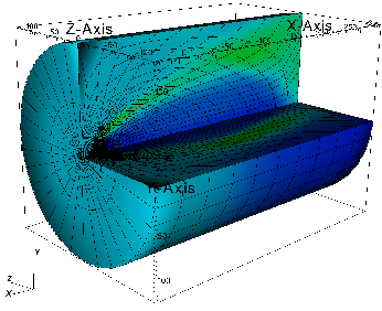
LFM Grid

The LFM uses a distorted spherical grid which is adapted to the magnetosphere. This is described in detail in the 2004 paper The Lyon-Fedder-Mobarry (LFM) global MHD magnetospheric simulation code.

The X_grid,Y_grid,Z_grid positions in the HDF file are in cartesian coordinates. Occasionally it is useful to work with the LFM grid in cylindrical coordinates. If you dig around the code much, you may see references to X2,Y2 and PHI. These are the LFM grid in cylindrical coordinates. The transformation to X2,Y2,PHI is:

x2(i,j) = x(i, j, 0) over all i,j
   y2(i,j) = y(i, j, 0) over all i,j
   phi(k) = atan2( z(10, 10, k), y(10, 10, k) ) for all k.

The LFM grid is aligned with the dipole axis. The dipole tilt is determined at runtime by the solar wind file: we assume that velocities are fed in in SM coordinates, which has the Z axis aligned with the dipole axis. The fact that the dipole is not aligned with the geographical axis is handled by the transformation of solar wind data from CSE or GSM coordinates to SM. In effect, the LFM fixes the dipole and rotate the universe around it.

How do I read data?

Several tools are available to read HDF4 LFM model output. The easiest is CISM_DX. Read below for more advanced methods of reading data.

C/C++

See example code in the repository at common/src/RMSerror/HDF_data.h

Fortran

See example code in the repository at LFM-para/src/hdftake-para.F.

IDL

NetCDF conversion

The NCAR Command Language (NCL) includes a utility to convert from HDF4 to NetCDF: ncl_convert2nc. See the NCL documentation for more information.

Python

See the Post-processing with Python page for details.