A simple plotting example for unstructured grid
Output from MUSICAv0 is on an unstructured grid (an unsorted vector of columns for defined latitude-longitude coordinates) making it difficult to visualize in standard plotting frameworks. NCAR has developed a small set of routines in Python as Jupyter notebooks that can be used for plotting results. A simple plotting routine with some examples is shown here:
#This first section of code is defining the modules we will be using and how they will be referenced in the code
import xarray as xr
import matplotlib.pyplot as plt
import numpy as np
import cartopy.crs as ccrs
import cartopy.feature as cfeature


#This section of code is defining the location of the result file(s) and extracting the relevant data
result_dir = "/glade/p/acom/MUSICA/results/opt_se_cslam_nov2019.FCHIST.ne0CONUSne30x8_ne0CONUSne30x8_mt12_pecount2700_SEACRS_TS1_CAMS_final_2013_branch/atm/hist/"
case_dir = "opt_se_cslam_nov2019.FCHIST.ne0CONUSne30x8_ne0CONUSne30x8_mt12_pecount2700_SEACRS_TS1_CAMS_final_2013_branch/atm/hist/"
result_file = "opt_se_cslam_nov2019.FCHIST.ne0CONUSne30x8_ne0CONUSne30x8_mt12_pecount2700_SEACRS_TS1_CAMS_final_2013_branch.cam.h0.2013-07.nc"
#here we are using xarray to read the defined netcdf file and writing into the variable nc
nc = xr.open_dataset(result_dir+case_dir+result_file)
#we can operate on nc now, so we are taking a slice at time 0 (first entry) and 32nd level (surface)
nc1 = nc.isel(time=0,lev=31)
#from this slice we will read the latitude (lat), longitude (lon), and ozone mixing ratio (O3)
lat = nc1['lat']
lon = nc1['lon']
var_mus = nc1['O3']


#To put data on a traditional fixed-grid we are using griddata
from scipy.interpolate import griddata
#this will define the lat/lon range we are using to correspond to 0.1x0.1 over CONUS
x = np.linspace(225,300,751)
y =  np.linspace(10,60,501)
#this will put lat and lon into arrays, something that is needed for plotting
X, Y = np.meshgrid(x,y)
#here we are putting the unstructured data onto our defined 0.1x0.1 grid using linear interpolation
grid_var = griddata((lon,lat), var_mus, (X, Y), method='linear')


#We can also put the previous statements into a function that can be called later in the notebook. This simplifies the variable selection and regridding.
def grid_musica(var, time, lev):
    nctmp = nc.isel(time=time, lev=lev)
    vartmp = nctmp[var]
    X, Y = np.meshgrid(x,y)
    grid_var = griddata((lon,lat), vartmp, (X, Y), method='linear')
    return grid_var


#To simplify plotting routines we are going to define a plotting function here
def plot_map_LCC(data, lat, lon, llim, ulim, units):
    #if you want to change the figure size of map projection you can do it here
    fig, ax = plt.subplots(figsize=(16, 9), subplot_kw=dict(projection=ccrs.LambertConformal()))
    #this is the actual plotting routine, using pcolormesh. Most variables are inputs from the function call
    im = ax.pcolormesh(lon,lat,data,cmap='Spectral_r',vmin=llim, vmax=ulim, transform=ccrs.PlateCarree())
    #this is for visualization of administrative boundaries. Many shapes included in the 'Natural Earth' library can also be used
    ax.coastlines(resolution='50m')
    ax.add_feature(cfeature.BORDERS)
    ax.add_feature(cfeature.STATES, edgecolor='#D3D3D3')
    cb = fig.colorbar(im, ax=ax)
    cb.set_label(units)
	return fig, ax


#Here you can see how the plotting function above is called in the notebook
fig, ax = plot_map_LCC(grid_var,Y,X,1e-8,1e-7,'mol/mol')
#we will zoom in slightly on the extents that are defined based on map projection
ax.set_extent([-32e5, 32e5, -25e5, 22e5], crs=ccrs.LambertConformal())
plt.title("Surface O$_{3}$ July 2013 MUSICAv0 Uniform Grid")


#this section shows how easy it can be to plot new variables/domains with functions
grid_var = grid_musica('CO',0,20)
fig, ax = plot_map_LCC(grid_var,Y,X,5e-8,1e-7,'mol/mol')
ax.set_extent([-32e5, 32e5, -25e5, 22e5], crs=ccrs.LambertConformal())
plt.title("525mb CO July 2013 MUSICAv0 Uniform Grid")
grid_var = grid_musica('CO',0,31)
fig, ax = plot_map_LCC(grid_var,Y,X,5e-8,2.5e-7,'mol/mol')
ax.set_extent([-32e5, 32e5, -25e5, 22e5], crs=ccrs.LambertConformal())
plt.title("Surface CO July 2013 MUSICAv0 Uniform Grid")
Using a pre-defined python module for plotting
For people who are not familiar with python, we have developed a python module that people can easily import and plot CAM-chem results (either structured or unstructured) with a single line command. First, download this python module for plotting (you may need to "right click" on the link and choose "Save link as..." from the menu, or find it here: https://github.com/NCAR/CAM-chem/blob/main/docs_sphinx/examples/functions/Plot_2D.py) and put it in your directory. If you are new to python, you need to know how to import a library, and you have to install required libraries for plotting (xarray, matplotlib, cartopy, etc.). See this python tutorial (or contents on this webpage) if you are new to python.
If you want reproduce the example plots below, download these files:
- structured grid (0.95 x 1.25) model output (sample.nc)
- unstructured grid (ne30x16) model output (sample_se.nc)
- SCRIP grid file for unstructured grid (sample_se_scrip.nc)
Of course, you can use your own CAM-chem history files instead of example files, unless you want to get the exactly same example plots below for checking.
NOTE: As of 10-MAR-2021, the Plot_2D script will be maintained in CAM-chem python Github. We shall keep examples here for reference, as those could still be helpful for beginners.
NOTE 2: As of 04-OCT-2021, the Plot_2D script can be installed using the PyPI package: https://pypi.org/project/vivaldi-a/
Preparation
First, you need to import built-in python libraries and Plot_2D module you just downloaded. Make sure Plot_2D.py file is in your directory.
import xarray as xr # To read NetCDF files
from Plot_2D import Plot_2D # To draw plots
import matplotlib.cm as cm # To change colormap used in plots
Let's read the model output files using the xarray module.
# FV file (structured grid)
fv_filename = "sample.nc"
ds_fv = xr.open_dataset( fv_filename )

# SE with regional refinement file (unstructured grid)
se_filename = "sample_se.nc"
ds_se = xr.open_dataset( se_filename )

# scrip filename for SE with regional refinement (contains grid information)
scrip_filename = "sample_se_scrip.nc"
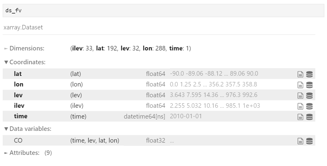
As a side note, you can check the variables in the file like below.
Plotting examples
To demonstrate the examples below, you will need to use Jupyter notebook. If you are using the local machine, Jupyter notebook is OK to use (https://jupyter.org/). However, if you use a separate server that needs remote access, you may want to install JupyterLab (https://jupyterlab.readthedocs.io/en/stable/) to use Jupyter notebook. You can still use Jupyter notebook on your server but it could be slow. If you are using Cheyenne or Casper machines, Jupyterhub is another option you can use (https://www2.cisl.ucar.edu/resources/jupyterhub-ncar). Jupyterhub is the easiest option you can start with if you are new to python, because you don't have to install python and required packages (already installed).
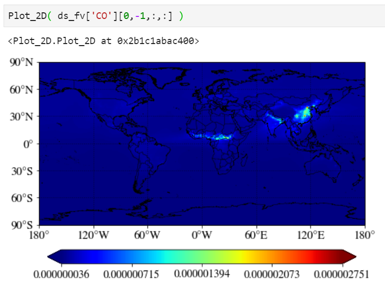
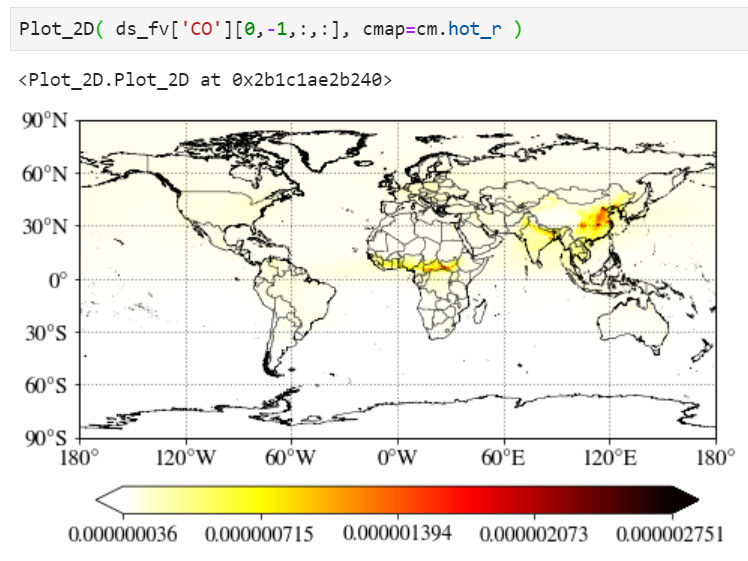
A simple plot
Just pass your surface CO. "-1" corresponds to the surface level as CESM writes the output from the top of the atmosphere to the surface.
Changing colormap
You can simply change the colormap with the "cmap" keyword. Check out this website for built-in colormaps in matplotlib python library.
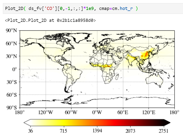
Multiplying scale factors
You can simply multiply any numbers (1e9 in the example below) in the input value.
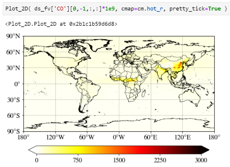
Pretty tick option
If you set pretty_tick=True, the routine will automatically find the colorbar ticks like below.
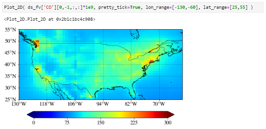
Plotting a region of interest only
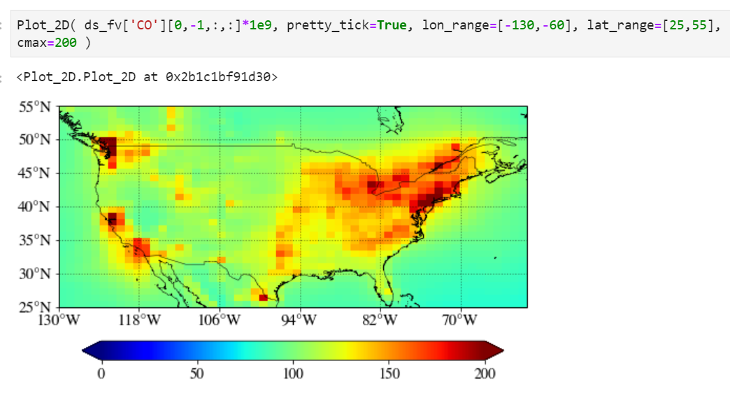
You can set "lon_range" and "lat_range" keywords to plot a region.
Setting maximum value for the plot
Use "cmax" keyword to force the maximum value to what you want.
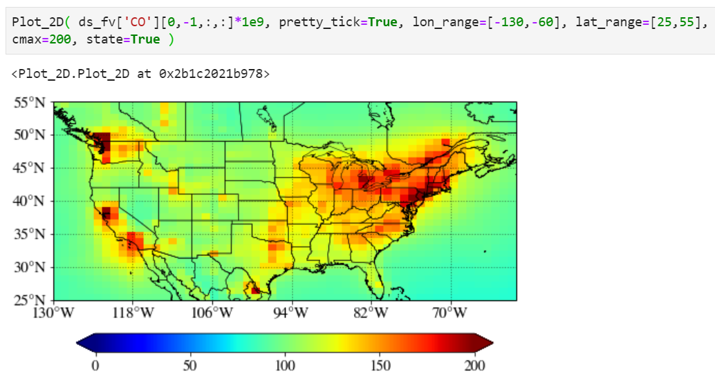
Adding state/province boundary lines
You can also easily add state boundary lines with the "state" keyword.
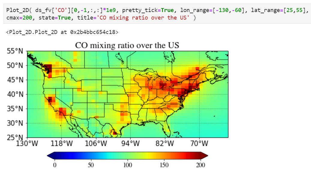
Adding a title in the plot
You can also add a title in the plot with a title keyword.
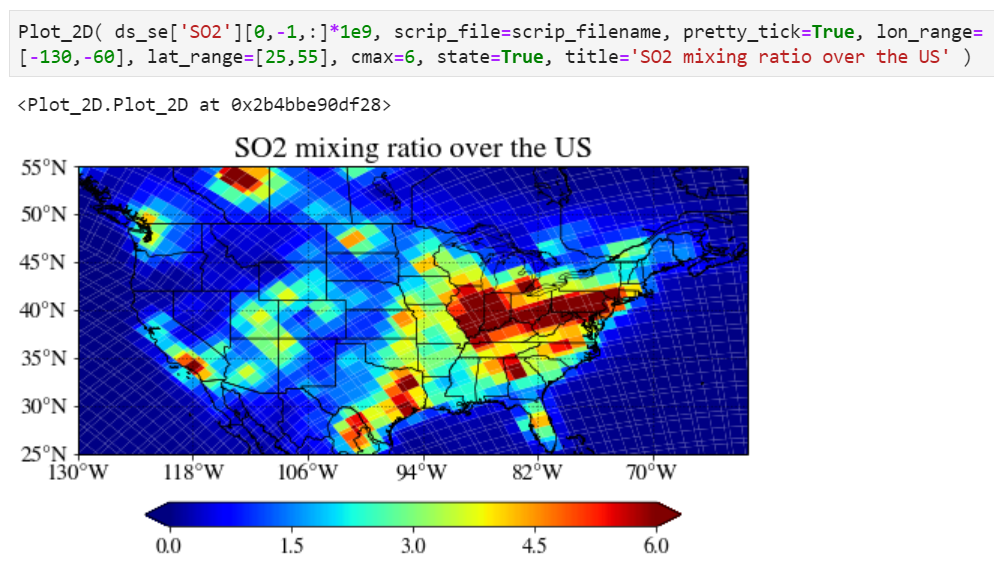
Plotting on unstructured grid
You can use exactly the same function and interface to plot unstructured grid model output.
The only difference is you have to specify the location of corresponding SCRIP grid file.
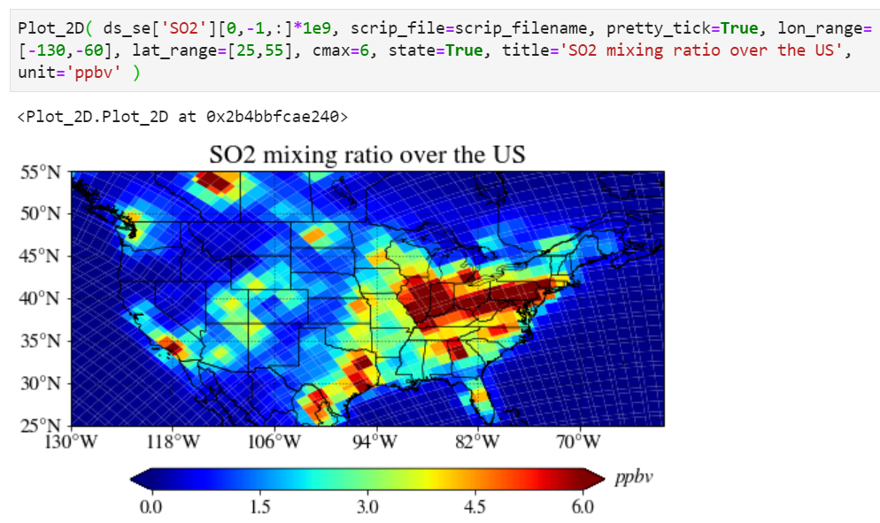
Adding a unit
You can add a unit with a unit keyword.
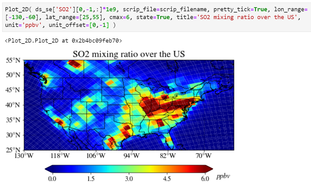
Adjusting unit position can also be done using the "unit_offset" keyword.
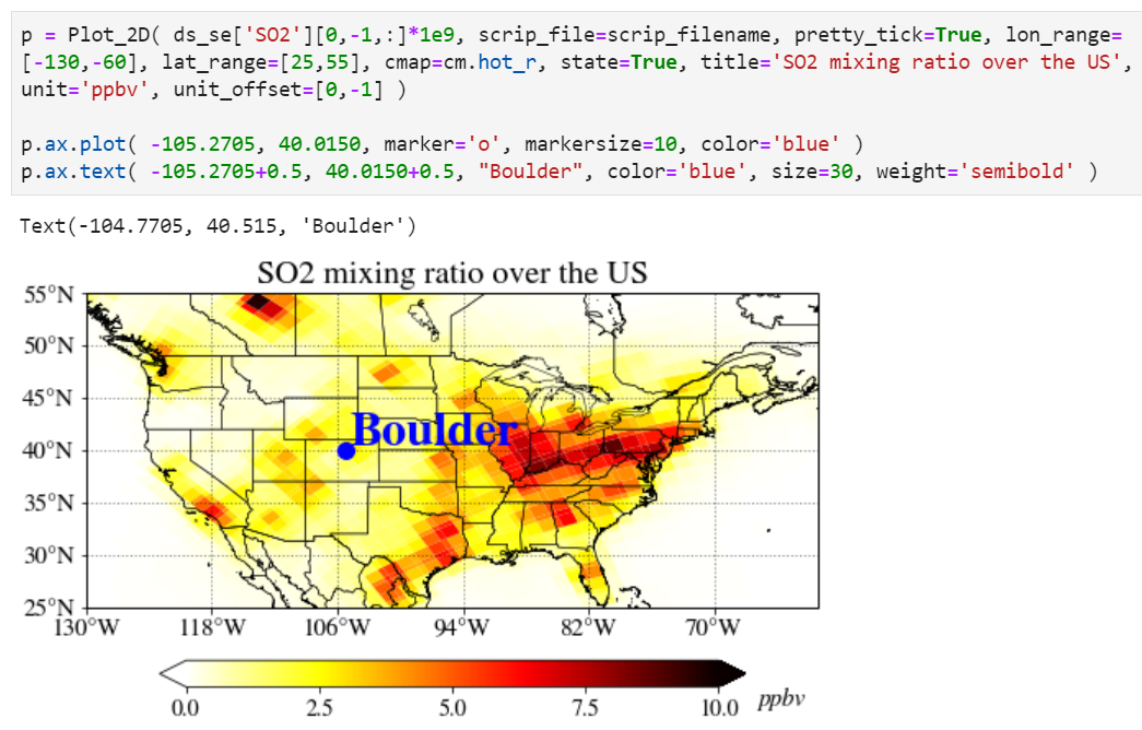
For advanced users: Adding more custom things you want
If you are an experienced user, you can add anything you want by getting an instance. As an example, we provide how to add a location point on top of the plot. Note "p = Plot_2D(...)" instead of "Plot_2D(...)", it creates a new instance of the class and assigns this object to the local variable "p".
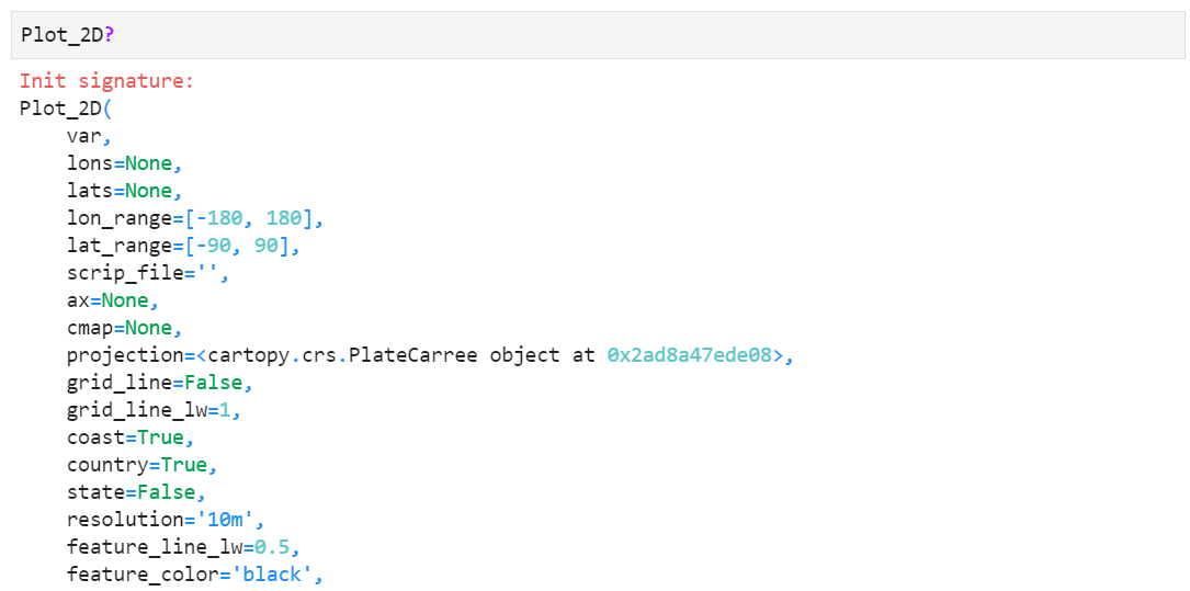
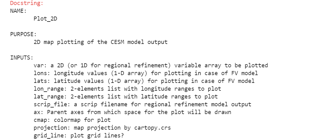
More custom options and keywords
There are a lot of custom options you can explore, such as changing map projections, grid line settings, coast/country/state lines, passing parent axes for multi-plot, colorbar orientation and size, etc. For more information, type "Plot_2D?" in your python or jupyter notebook shell prompt. You will find detailed information of each keyword like below.