According to the Licor 7500 manual, there is a 0.186 second sampling lag in the 7500. This can be increased with an output delay parameter, so that it can be synchronized with the sampling of a sonic. I've verified that the output delays on our 7500's are set to 0.
Since the CSAT3 and Licor operate asynchronously, I see no advantage in further adjustment of the Licor delay to be a multiple of the CSAT3 sample period.
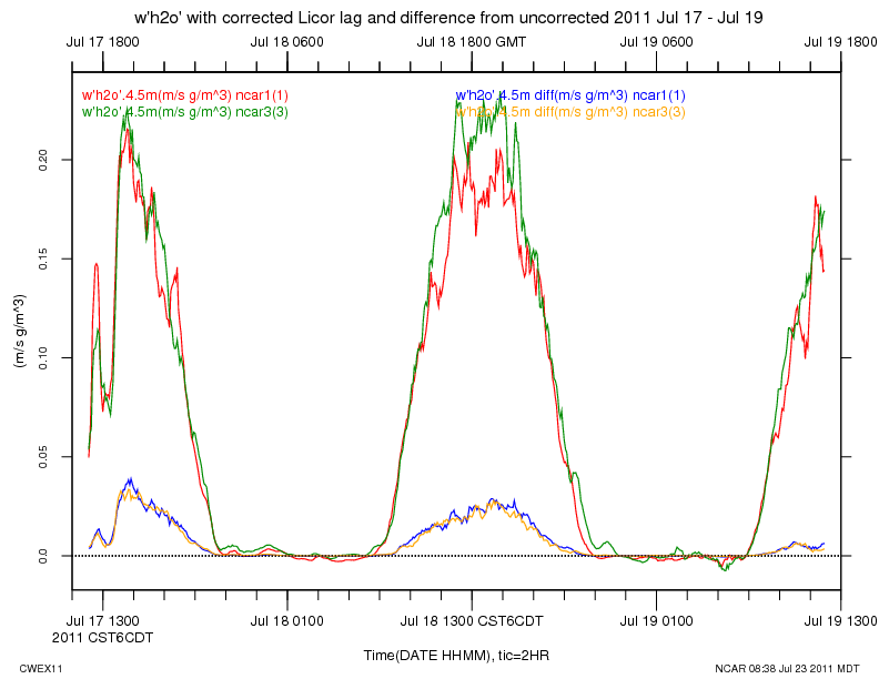
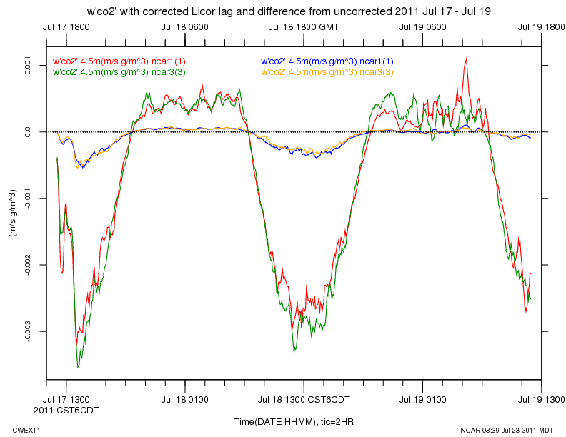
We have not been incorporating a 7500 lag in our data processing. We do correct for the 2 sample delay of the CSAT3 sonics. Subtracting 0.186 seconds from the 7500 samples does increase the correlation and fluxes between w and h2o and co2. The w'h2o' and w'co2' fluxes increase by about 15% when a lag of 0.186 is applied to the Licor data. These plots are of the corrected flux and the difference between the corrected and uncorrected fluxes, for 2 days, centered on Jul 18:
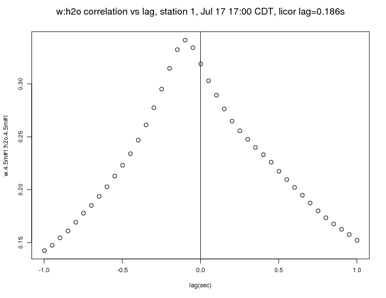
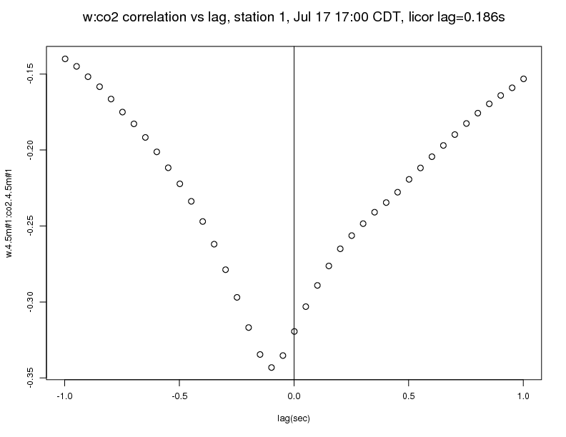
Here are the correlation vs lag plots between w and h2o and co2 from station 1 for Jul 17, 17:00 - 17:30 CDT. The wind was out of the south at this time:
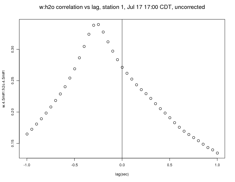
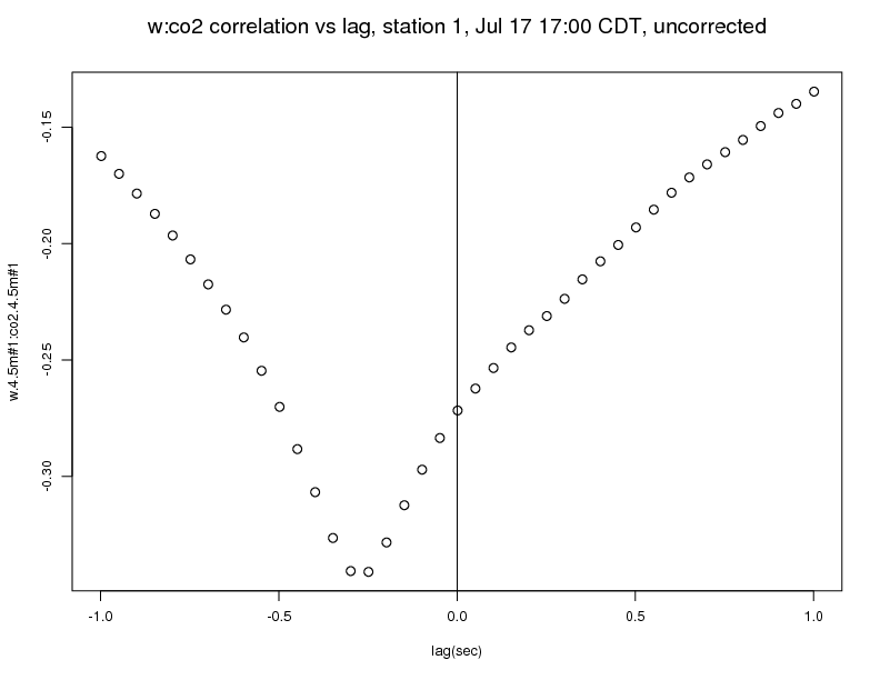
After applying a 0.186 second lag to the Licor data, you can see that the correction is in the right direction, but there is still a lag of about 2 samples, 0.1 seconds:
(It pays to read the manual!)
For future reference, here is the splus code to plot the correlations:
dpar(start="2011 jul 17 17:00",lenmin=30,stns=1)
iod = prep(c("w.4.5m#1","h2o.4.5m#1","co2.4.5m#1"),rate=20)
x = readts(iod)
close(iod)
cwh = crosscorr(x[,1:2],lags=c(-1,1))
plot(as.numeric(utime(positions(cwh))),cwh,xlab="lag(sec)",ylab="w.4.5m#1:co2.4.5m#1")