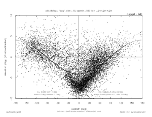
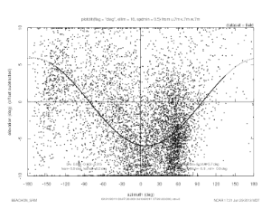
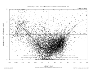
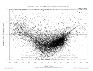
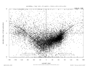
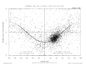
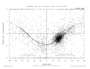
The following plots were made with our Splus function, plot.tilt, that does a linear least squares fit to find the plane of mean flow, and plots the wind vector elevation angle vs azimuth. The planar fit becomes a sine curve on the tilt plot.
See EOL sonic tilt documentation.
From a long term plot of the sonic "diag" value, I chose two periods where the the values were consistently very small. plot.tilt discards 5 minute wind averages when "diag" is above 0.01, or more than 1% of the data has a non-zero CSAT3 diagnostic value.
For the upper sonics at 16, 30 and 43 meters, the minimum wind speed used for the fit was 1.0 m/s. For the lower sonics at 2 and 7 meters, the minimum wind speed was set to 0.5 m/s. This didn't have much effect on the fit, however.
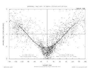
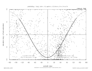
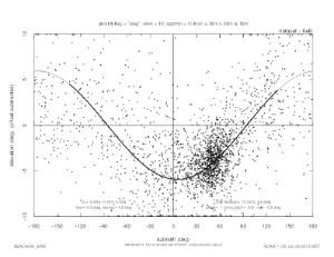
Feb 21 to April 4, 2011
2 meters
7 meters
16 meters
30 meters
43 meters
Aug 5 to Aug 17, 2011
date |
height (m) |
lean |
leanaz |
w offset (m/s) |
elevation residual rms (deg) |
offset residual rms (m/s) |
notes |
|---|---|---|---|---|---|---|---|
Feb-Apr 2011 |
2 |
4.1 |
-1.7 |
0.03 |
2.9 |
0.04 |
|
|
7 |
5.9 |
8.2 |
0.07 |
5.7 |
0.08 |
|
|
16 |
5.9 |
-0.2 |
-0.01 |
3.1 |
0.011 |
|
|
30 |
4.5 |
-2.1 |
0.02 |
2.7 |
0.014 |
|
|
43 |
4.3 |
-5.9 |
0.04 |
3 |
0.02 |
|
Aug 2011 |
2 |
5.6 |
-6.3 |
0.04 |
2.6 |
0.03 |
|
|
7 |
9.1 |
-1.4 |
0.06 |
7 |
0.09 |
large tilt value, too much scatter for good fit |
|
16 |
5.9 |
4.6 |
-0.01 |
3.6 |
0.01 |
|
|
30 |
4.3 |
-0.9 |
0.00 |
3.6 |
0.01 |
|
|
43 |
4.4 |
-5.5 |
0.01 |
4.2 |
0.02 |
|
Tom says that typical droop of sonic booms results in 1 to 2 degree tilts. The sonic booms point up-slope from the tower, so the approximate 5 degree tilts seen here are a combination of the boom "droop" and the slope of the terrain.
They generally agree on an approximate 5 degree tilt of the sonics relative to the mean flow, except the 9.9 degree tilt for the 7m sonic in Aug 2011.
There appears to be some local "disturbance in the force", causing a pinched effect at 2 meters, and to a lesser extent at 7 meters, so that winds straight into the sonic have an additional downward inclination.
There seems to be good agreement at 16 meters and above between the two fits. I suggest using the average of the two values for those levels. Perhaps we need to look at more data for 2 and 7 meters.
dpar(start="2011 2 21 00:25",end="2011 4 4 07:26",coords="instrument")
dpar(hts=2)
plot.tilt(flag="diag",ellim=10,spdmin=0.5)