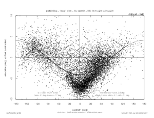
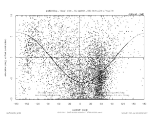
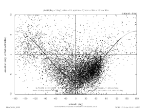
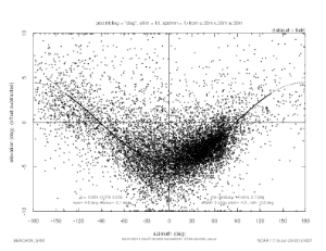
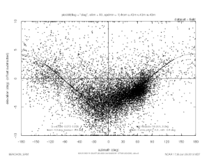
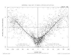
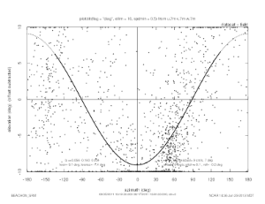
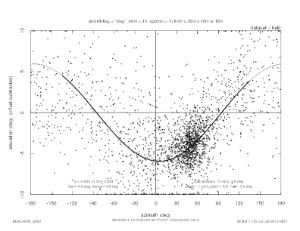
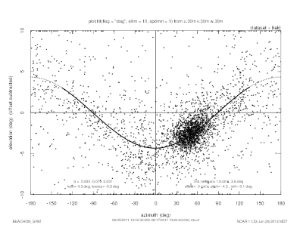
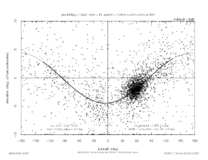
The attached following plots were made with our Splus function, plot.tilt, that does a linear least squares fit to find the plane of mean flow, and plots the wind vector elevation angle vs azimuth. The planar fit becomes a sine wave on the tilt plot.
...
For the upper sonics at 16, 30 and 43 meters, the minimum wind speed used for the fit was 1.0 m/s. For the lower sonics at 2 and 7 meters, the minimum wind speed was set to 0.5 m/s. This didn't have much effect on the fit, however.
Feb 21 to April 4, 2011
| Section | ||||||||||
|---|---|---|---|---|---|---|---|---|---|---|
| ||||||||||
|
Aug 5 to Aug 17, 2011
| Section | ||||||||||
|---|---|---|---|---|---|---|---|---|---|---|
| ||||||||||
|
date | height (m) | lean | leanaz | w offset (m/s) | elevation residual rms (deg) | offset residual rms (m/s) | notes |
|---|---|---|---|---|---|---|---|
Mar 2011 | 2 | 4.1 | -1.7 | 0.03 | 2.9 | 0.04 |
|
| 7 | 5.9 | 8.2 | 0.07 | 5.7 | 0.08 |
|
| 16 | 5.9 | -0.2 | -0.01 | 3.1 | 0.011 |
|
| 30 | 4.5 | -2.1 | 0.02 | 2.7 | 0.014 |
|
| 43 | 4.3 | -5.9 | 0.04 | 3 | 0.02 |
|
Aug 2011 | 2 | 5.6 | -6.3 | 0.04 | 2.6 | 0.03 |
|
| 7 | 9.1 | -1.4 | 0.06 | 7 | 0.09 | large tilt |
| 16 | 5.9 | 4.6 | -0.01 | 3.6 | 0.01 |
|
| 30 | 4.3 | -0.9 | 0.00 | 3.6 | 0.01 |
|
| 43 | 4.4 | -5.5 | 0.01 | 4.2 | 0.02 |
|
...
These tilts appear to be due to the slope of the terrain, which is downward in the -u direction, in the direction that the sonic boom points. If the terrain was not sloping, these would be a "backwards" boom tilt, i.e. the booms not drooping from the tower but angling upward. They generally agree on an approximate 5 degree slope of the terrain relative to the sonics, except the 9.9 degree tilt for the 7m sonic in Aug 2011.
| Gallery | ||||||
|---|---|---|---|---|---|---|
|
...
| Code Block | ||
|---|---|---|
| ||
dpar(start="2011 2 21 00:25",end="2011 4 4 07:26",coords="instrument") dpar(hts=2) plot.tilt(flag="diag",ellim=10,spdmin=0.5) |