Current status: IN TRUNK
Code is currently in the trunk and will be publicly released in the next round of major update. We have tested OASISS for a number of compounds, including acetaldehyde (CH3CHO), 1 acetone (CH3COCH3), 2 organohalogens (e.g. CHBr3, CH2Br2), 3 and dimethyl sulfide (DMS), using a combination of airborne, ship-borne and satellite observations.
Point of contact: Siyuan Wang | NOAA
OVERVIEW
The ocean emits a wide range of climate-relevant gases. Most chemistry-climate models use prescribed emissions, which is simple and straightforward. But prescribed emissions usually do not respond to changes in local conditions. In this wiki we describe a new Online Air-Sea Interface for Soluble Species (OASISS) is developed for CESM | CAM-Chem to calculate the bi-directional oceanic fluxes of trace gases of interest. In brief, this model determines the direction and the magnitude of the ocean fluxes based on solubility, the physical conditions in the ocean (e.g., sea surface temperature, salinity, waves and bubbles) and the atmosphere (temperature, wind). This module is fully coupled with atmospheric chemistry and dynamics as well.
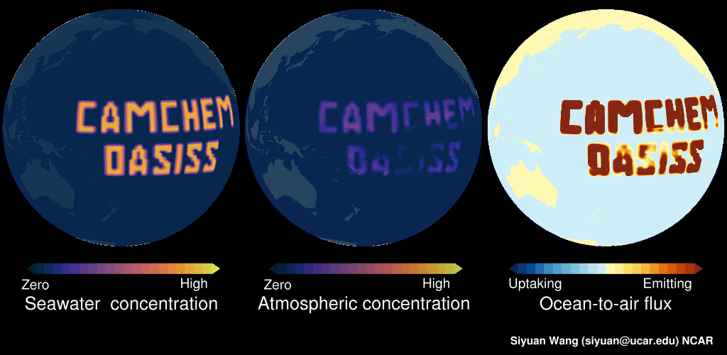
Please see this demo: LEFT panel shows the surface seawater concentration of an imaginary gas (in this example, constant surface seawater concentration is prescribed in the middle of Pacific). The MIDDLE panel shows the CAM-chem predicted surface atmospheric concentration, as you can see this compound is dispersed in the atmosphere. The RIGHT panel shows the ocean-to-air flux, with warmer colors indicating net emitting and colder colors indicating net uptake. In regions with high seawater concentrations, the surface seawater is supersaturated, and hence the ocean is net emitting. But in near-by regions with low surface seawater concentrations, the surface seawater is undersaturated, and the ocean is net uptaking. Note: no chemicals were actually released into the Pacific in making this video!
BRIEF INTRODUCTION
This module is mainly based on the two-layer model as previously described. 4 The air-sea flux is calculated from the concentration gradient across the air-sea interface, as well as the transfer velocities on the air-side (kair, in s-1) and water-side (kwater, in s-1). kair is mainly based on the NOAA COARE algorithm, 5 with the addition of the still air diffusive flux adjustment. 6 kwater is based on Nightingale et al. 7 In addition, the bubble-mediated transfer 8 is included in the air-sea exchange module, in which the fractional coverage of actively breaking whitecaps is parameterized based on previous study. 9 The bubble-mediated transfer is optional, i.e. user can switch this on or off in $caseroot/user_nl_cam.
USER INPUT
Surface seawater concentration (nanomoles per liter) of the species of interest and surface seawater salinity (parts per thousand) need to be provided in $caseroot/user_nl_cam. For example:
$CASEROOT/user_nl_cam | |
|---|---|
0 1 2 3 4 | bubble_mediated_transfer = .FALSE.ocean_salinity_file = '/$your_directory/$salinity_file.nc'csw_specifier = 'Species_1 -> Scaling_Factor * /$your_directory/$seawater_concentration_for_Species_1_in_nanomole_per_liter.nc', 'Species_2 -> Scaling_Factor * /$your_directory/$seawater_concentration_for_Species_2_in_nanomole_per_liter.nc'csw_time_type = 'SERIAL' |
The chemistry package reads in seawater concentration data from netCDF files. Each tracer species is read from its own file as directed by the namelist variable CSW_SPECIFIER (Line 2-3). This is similar to emis_specifier. SCALING_FACTOR (Line 2 and 3) is exactly what it looks like. This is optional. Default (omit) is1.0. CSW_TIME_TYPE (Line 4): type of time interpolation of seawater concentration datasets specified. Valid values: CYCLICAL,SERIAL,INTERP_MISSING_MONTHS,FIXED.
The seawater concentration fields can be read in as time series of data, cycle over a given year, or be fixed to a given date. For example, to specify cycle year of the seawater concentration data:
$CASEROOT/user_nl_cam | |
|---|---|
4 5 | csw_time_type = 'CYCLICAL'csw_cycle_yr = 2016 |
The input data (salinity and surface seawater concentrations) must be the same horizontal resolution as the model configuration. The surface seawater concentration files must cover the entire simulation time period also - better have a short "grace period" after the end of the model end date.
The calculated emissions fluxes, salinity and seawater concentrations can be saved in output in variables:
$CASEROOT/user_nl_cam | |
|---|---|
6 | fincl2 = 'OCN_FLUX_DMS', 'OCN_FLUX_CH3CHO', 'OCN_FLUX_CH3COCH3', ! emissions fluxes |
NOTE: The ocean emissions are NOT included in the SF{species} output variables.
UNDER THE HOOD
In this framework, the air-sea exchange of a given soluble gas is determined by (i) solubility; (ii) kinetics; and (iii) concentration gradient at the interface. The solubility (effective Henry's law constant) is given in the FORTRAN source code, and the kinetics (e.g., the transfer velocities) will be calculated based on local physical forcing in the ocean and the atmosphere. The concentration in the atmosphere is explicitly solved in the atmospheric model, the local surface seawater concentration, ideally, should be explicitly solved in the ocean model. Unfortunately, for most of the trace gases of interest, the ocean biogeochemical processes affecting the sources and sinks in the seawater remain unclear. Therefore user needs to provide the input surface seawater concentration fields.
There are a couple of ways to construct the surface seawater concentration fields. For example, fixed concentrations, or simple latitude-dependent concentrations can be used. In the case of acetaldehyde (CH3CHO), a satellite-based approach (similar to Millet et al 10 ) is used to estimate the average concentration in the ocean mixed layer. In brief, the production of acetaldehyde from the photolysis of the colored dissolved organic matter is estimate using the NASA SeaWiFS level-3 monthly climatology of absorption coefficient due to colored dissolved and detrital organic matter at 433 nm. This approach reasonably captures the large-scale features as revealed from ship-based observations.
Recently, I have developed an observationally trained machine-learning emulator, which couples the ocean biogeochemistry with the air-sea exchange. An observational dataset, including the surface seawater concentration of any compound of interest, is needed to train the machine-learning algorithm, which will then predict the global surface seawater concentration fields of this compound. The training dataset has to be sufficiently comprehensive, e.g., should cover a variety of global ocean regimes and different seasons / months as well. Currently I am using this machine-learning approach for the brominated very short-lived substance (CHBr3 and CH2Br2) 3 and dimethyl sulfide (DMS). The machine-learning emulator is capable of capturing the spatial and temporal distributions of CHBr3 and CH2Br2 in the surface seawater (evaluated with HALOCAT dataset), long-term global surface observations (NOAA/ESRL global monitoring network), and global-scale, multiseasonal airborne measurements (NASA ATom) 3 Please contact me if you are interested.
EXAMPLE: DMS
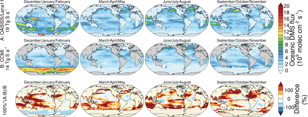
Most models use prescribed oceanic emission fluxes (offline) for DMS, which is less skillful since the prescribed emission fluxes are decoupled from the meteorology, atmospheric chemistry and dynamics. Over the past decades, more and more seawater DMS measurements become available, making it possible to derive observation-based surface seawater concentration product. Such surface seawater concentration fields can be used to drive the air-sea exchange of DMS. A brief test using the surface seawater DMS climatology in Lana et al. (2011) 11 is presented here, and compared to the CCMI oceanic DMS emission that is used in CESM for CMIP6 (which is from Kettle and Andreae, 2000). As shown in the plot below, the OASISS + Lana et al. (2011) configuration yields an annual oceanic DMS emission of 19 Tg S a-1, which is 33% higher than the DMS emission from CCMI (14 Tg S a-1).
A few notes:
OASISS + Lana et al. (2011) DMS emission (19 Tg S a-1) is comparable to the recent literature but maybe towards the lower end of the earlier studies: 24 Tg S a-1 (Lennartz et al. 2015 12 ); 16-20 Tg-S/year (Gale et al. 2018 13 ); 15-33 Tg-S/year (Kettle and Andreae 2000 14 ). The difference among these can be partially explained by the transfer velocity parameterization. In OASISS, Nightingale (2000) 7 is used, and previous studies have used others, such as Wanninkhof (1992), 15 Erickson (1993). 16 This can cause some difference, see discussions in Kettle and Andreae (2000).
The annual DMS emission in our OASISS + Lana et al. (2011) configuration (19 Tg S a-1) is 32% lower than the flux calculated in Lana et al. (2011, 28 Tg S a-1). Both are using water-side resistance from Nightingale (2000). However, Lana et al. (2011) did not include the air-side resistance, which is generally considered not important for DMS but can be substantial when cold & high wind. This may explain some difference. Moreover, Lana et al. (2011) calculated the global DMS emission with zero DMS in the atmosphere, but OASISS is fully coupled with chemistry and dynamics. A quick test with zero DMS in the air in OASISS leads to 21 Tg S a-1 (some 10% higher) DMS emission. This makes sense, since elevated DMS in the atmosphere leads to a weaker sea-to-air flux (may even push the flux downward if air concentration is high enough). Lennartz et al. (2015) 12 reported a similar trend as well.
REFERENCES
- Wang, S., Hornbrook, R. S., Hills, A., Emmons, L. K., Tilmes, S., Lamarque, J.‐F., et al ( 2019). Atmospheric Acetaldehyde: Importance of Air‐Sea Exchange and a Missing Source in the Remote Troposphere. Geophysical Research Letters, 46. https://doi.org/10.1029/2019GL082034 ↩
- , , , , , , et al. (2020). Global Atmospheric Budget of Acetone: Air‐Sea Exchange and the Contribution to Hydroxyl Radicals. Journal of Geophysical Research: Atmospheres, 125, e2020JD032553. https://doi.org/10.1029/2020JD032553 ↩
- Wang, S., Kinnison, D., Montzka, S. A., Apel, E. C., Hornbrook, R. S., Hills, A. J., Blake, D. R., Barletta, B., Meinardi, S., Sweeney, C., Moore, F., Long, M., Saiz‐Lopez, A., Fernandez, R. P., Tilmes, S., Emmons, L. K., Lamarque, J-F. (2019). Ocean Biogeochemistry Control on the Marine Emissions of Brominated Very Short‐Lived Ozone‐Depleting Substances: A Machine‐Learning Approach. Journal of Geophysical Research - Atmospheres, 124, 12319– 12339. https://doi.org/10.1029/2019JD031288 ↩ ↩ ↩
- Johnson, M. T. (2010). A numerical scheme to calculate temperature and salinity dependent air-water transfer velocities for any gas. Ocean Sci., 6(4), 913–932. ↩
- Jeffery, C. D., Robinson, I. S., & Woolf, D. K. (2010). Tuning a physically-based model of the air–sea gas transfer velocity. Ocean Modelling, 31(1), 28–35. ↩
- Mackay, D., & Yeun, A. T. K. (1983). Mass transfer coefficient correlations for volatilization of organic solutes from water. Environmental Science & Technology, 17(4), 211–217. ↩
- Nightingale, P. D., Malin, G., S, L. C., Watson, A. J., Liss, P. S., Liddicoat, M. I., et al. (2000). In situ evaluation of air‐sea gas exchange parameterizations using novel conservative and volatile tracers. Global Biogeochemical Cycles, 14(1), 373–387. ↩ ↩
- Asher, W., & Wanninkhof, R. (1998). The effect of bubble‐mediated gas transfer on purposeful dual‐gaseous tracer experiments. Journal of Geophysical Research: Oceans, 103(C5), 10555–10560. ↩
- Soloviev, A., & Schluessel, P. (2002). A Model of Air-Sea Gas Exchange Incorporating the Physics of the Turbulent Boundary Layer and the Properties of the Sea Surface. Washington DC American Geophysical Union Geophysical Monograph Series, 141–146. ↩
- Millet, D. B., Guenther, A., Siegel, D. A., Nelson, N. B., Singh, H. B., de Gouw, J. A., Warneke, C., Williams, J., Eerdekens, G., Sinha, V., Karl, T., Flocke, F., Apel, E., Riemer, D. D., Palmer, P. I., and Barkley, M. (2010) Global atmospheric budget of acetaldehyde: 3-D model analysis and constraints from in-situ and satellite observations, Atmos. Chem. Phys., 10, 3405-3425, https://doi.org/10.5194/acp-10-3405-2010. ↩
- , et al. (2011), An updated climatology of surface dimethlysulfide concentrations and emission fluxes in the global ocean, Global Biogeochem. Cycles, 25, GB1004, doi:10.1029/2010GB003850. ↩
- Lennartz, S. T., Krysztofiak, G., Marandino, C. A., Sinnhuber, B.-M., Tegtmeier, S., Ziska, F., Hossaini, R., Krüger, K., Montzka, S. A., Atlas, E., Oram, D. E., Keber, T., Bönisch, H., and Quack, B.: Modelling marine emissions and atmospheric distributions of halocarbons and dimethyl sulfide: the influence of prescribed water concentration vs. prescribed emissions, Atmos. Chem. Phys., 15, 11753–11772, https://doi.org/10.5194/acp-15-11753-2015, 2015. ↩ ↩
- Galí, M., Levasseur, M., Devred, E., Simó, R., and Babin, M.: Sea-surface dimethylsulfide (DMS) concentration from satellite data at global and regional scales, Biogeosciences, 15, 3497–3519, https://doi.org/10.5194/bg-15-3497-2018, 2018. ↩
- , and (2000), Flux of dimethylsulfide from the oceans: A comparison of updated data sets and flux models, J. Geophys. Res., 105( D22), 26793– 26808, doi:10.1029/2000JD900252. ↩
- (1992), Relationship between wind speed and gas exchange over the ocean, J. Geophys. Res., 97( C5), 7373– 7382, doi:10.1029/92JC00188. ↩
- (1993), A stability dependent theory for air‐sea gas exchange, J. Geophys. Res., 98( C5), 8471– 8488, doi:10.1029/93JC00039. ↩
(Webpage currently under construction)
(This wiki architecture unfortunately doesn't appear to be entirely mobile-friendly)