Introduction
VisIt is a free interactive parallel visualization and graphical analysis tool for viewing scientific data on Unix and PC platforms. Users can quickly generate visualizations from their data, animate them through time, manipulate them, and save the resulting images for presentations. VisIt contains a rich set of visualization features so that you can view your data in a variety of ways. It can be used to visualize scalar and vector fields defined on two- and three-dimensional (2D and 3D) structured and unstructured meshes. For more information, you can check out this VisIt official website. In this page, we will look through how to use VisIt for MUSICA output plotting as a step-by-step process.
Pros and Cons (compared to IDL, python, NCL, etc.)
VisIt has a very interactive interface, so you can easily modify the plot including colorbar, annotations (texts or lines), regional zoom in/out, min/max/scale, etc. You don't have to rerun the code if you want to make a simple adjustment for your plot. You can also effortlessly do several things that you can't easily do in your command line language-based interface, such as picking up a value/info in the plot, changing a map projection, setting threshold values, and 3D plotting, etc.
However, because it is based on a graphical user interface, it is not good for an auto-script or generation of many plots, although VisIt supports a command-line interface based on python. If you are familiar with Igor Pro, the pros and cons of VisIt are similar to those of Igor Pro.
Installing VisIt
VisIt runs on the following platforms:
- Linux (including Ubuntu, RedHat, SUSE, TOSS)
- Mac OSX
- Microsoft Windows
You can install Visit on your personal computer, or you can use Visit on Cheyenne or Casper if you have an account (How to Get an account on Cheyenne).
See this page on VisIt User Manual for further instructions about how to install Visit on your machine, or just move to the next section if you want to use VisIt that already installed on the NCAR Cheyenne/Casper machines.
Starting VisIt
This section is for users who have access to NCAR Cheyenne/Casper server. You can skip this section if you already installed VisIt on your local machine above.
On Cheyenne
See this page provided by CISL to use Visit on Cheyenne: https://www2.cisl.ucar.edu/resources/computational-systems/cheyenne/software/starting-visit-cheyenne
On Casper
You can launch VisIt on Casper, by typing
casper%module load visit
casper%visit
It can be very slow if you run VisIt in the SSH terminal, as VisIt uses a graphical interface. You may want to use VNC instead. You can find how to use VNC on Casper: https://www2.cisl.ucar.edu/resources/computational-systems/casper/using-remote-desktops-casper-vnc
Basic plotting with global finite volume CAM-chem output
Here we will show how to make a 2D global map plot using VisIt graphical interface. For a deeper understanding of VisIt, you can see the official VisIt tutorial first, although we will go through the processes thoroughly. Download a sample NetCDF file for hands-on instructions below.
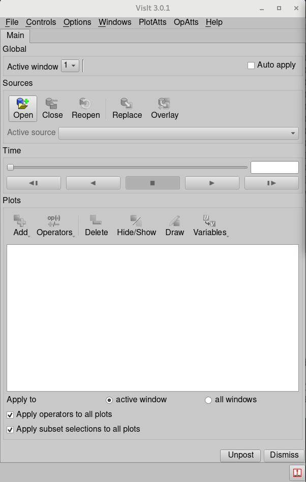
Opening a file
- Go to the GUI and click on the Open icon.
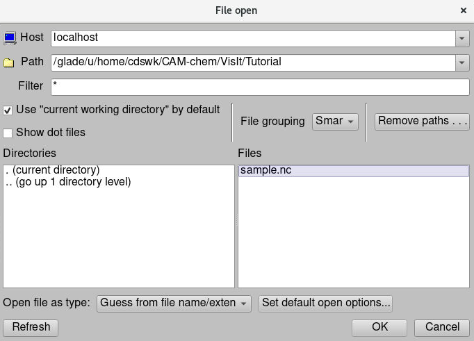
- This brings up the File open window.
- Change the Path field to the folder that has sample.nc file that you downloaded above.
- Highlight the file "sample.nc" and then click OK.
You can change GUI style (e.g., color, size, font) by selecting "Options" → "Appearance"
Making a plot
- Click on the Add icon to access various plots. This is located about half way down the Main window.
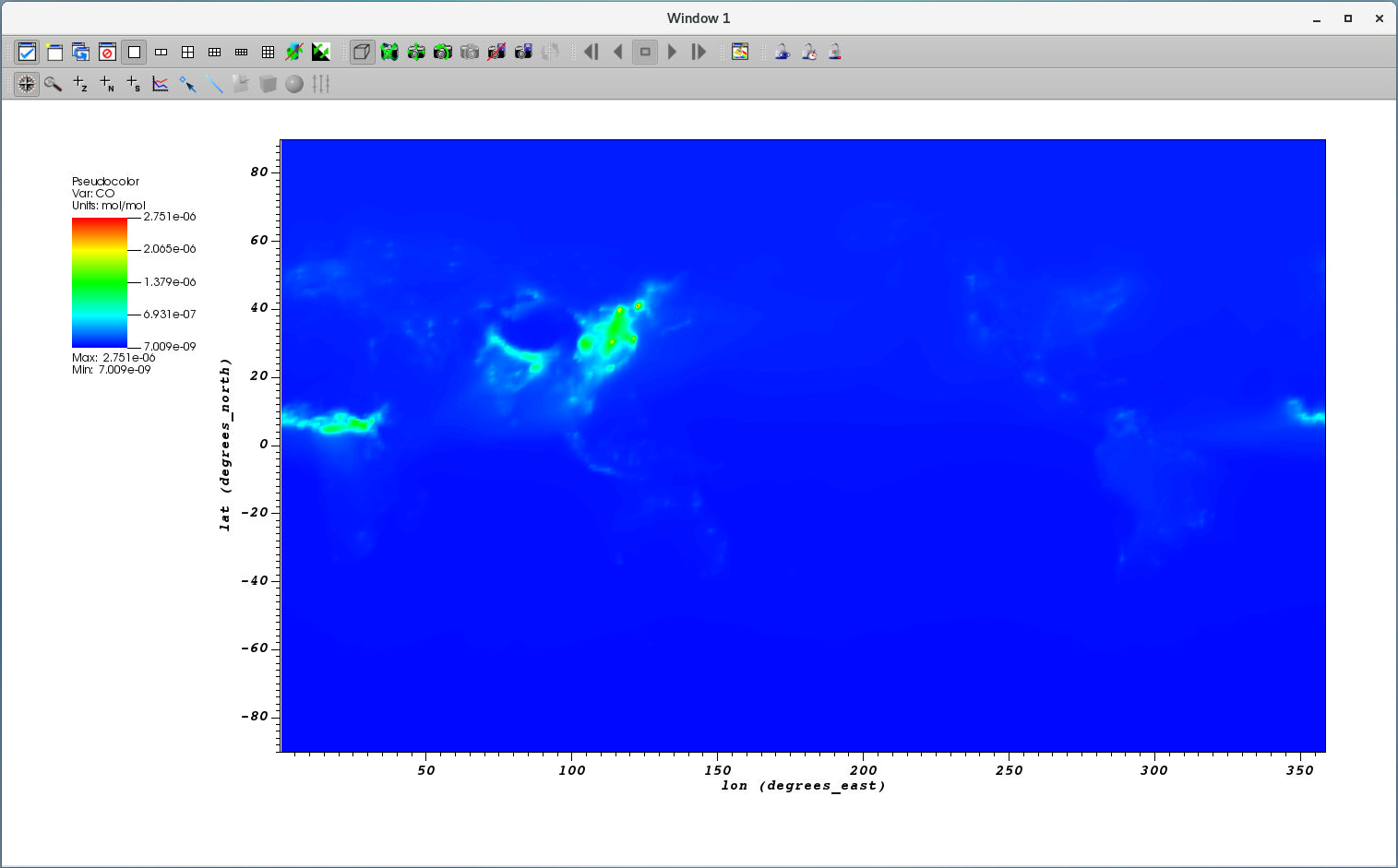
- Select Pseudocolor → "CO" to add a Pseudocolor plot.
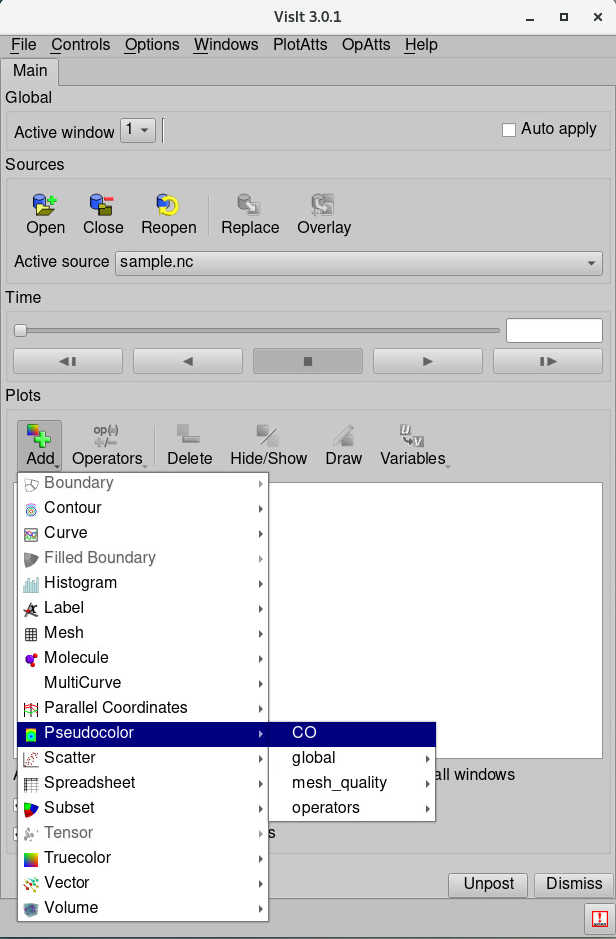
- After adding a plot, you will see a green entry added to the "Plot list", which is located half way down the GUI.
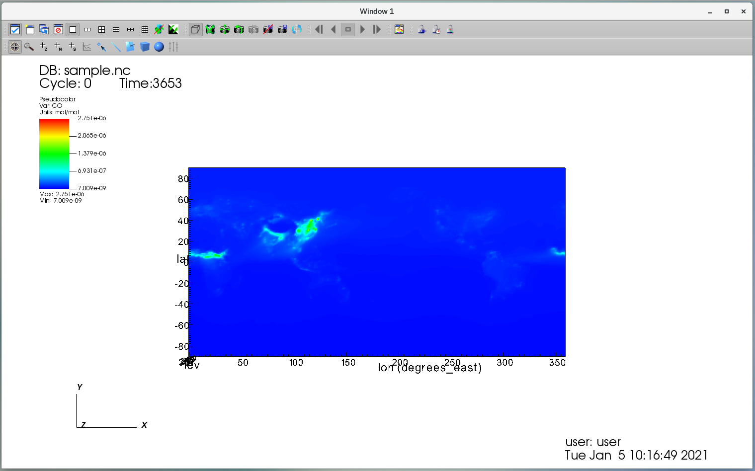
- Click Draw.
- You should see a plot appear in the visualization window.
Making a 2D plot using a Slice operator
What you can see is actually a 3D plot (top-down view) because the CO variable has three dimensions - (lev,lat,lon). You can check it by clicking the left mouse button and dragging with the mouse, which will perform an action that moves and rotates (like the video below).
Now let's make a 2D plot for the surface.
- Click on the Operators icon.
- Select Slicing --> Slice to add a slice operator.
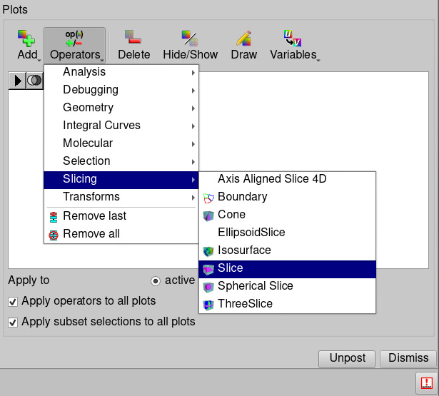
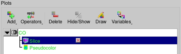
- Click ▶ icon to see an added operator.
- Double-click on the Slice or select menu OpAtts --> Slicing --> Slice
- We want the slice plane to be along the Z-axis, so click the Z-Axis radio button.
- For CAM-chem 32 layer model, a vertical index of 31 is the surface (0 is a model-top). Click the Intercept radio button and put the number 31.
- Click Apply to change Slice properties.
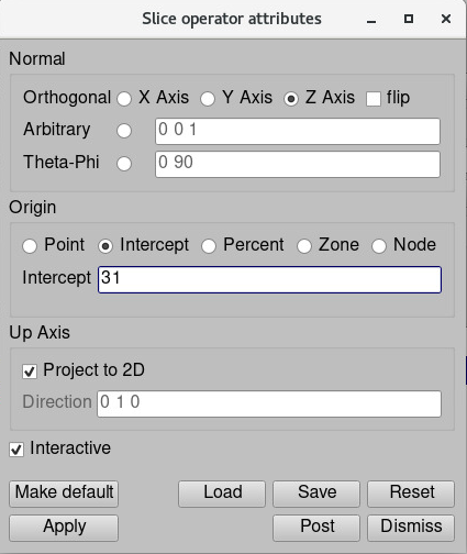
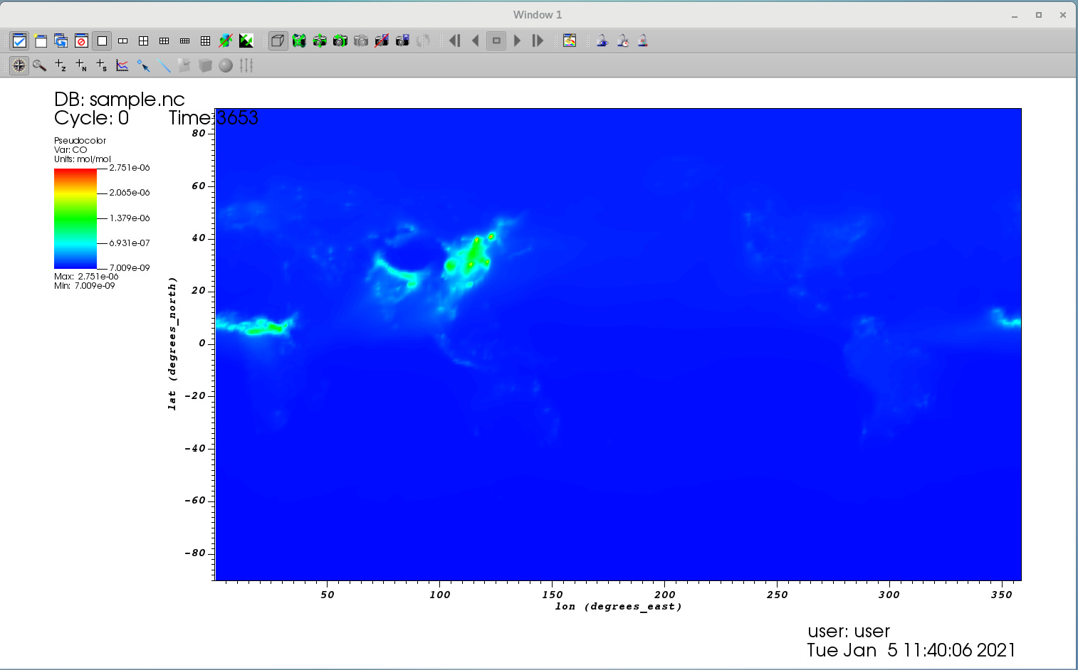
- Click Draw to make the plot.
- Now you can see more clear plot (no axis for lev).
- For more information, see this manual website about Slice operator
Adjusting annotations
There are several annotations in the plot (e.g., texts in the upper left and lower right) that you may want to remove.
- Open Annotation window. Select Controls --> Annotation.
- If you uncheck Legend, the colorbar will disappear.
- Uncheck Database to remove texts in the upper left.
- Uncheck User Information to remove texts in the lower right.
- Click Apply.

- Now you can see more clear plot (no redundant information)
- For more information, see this manual website about Annotations
Adjusting colorbar (position, size, orientation, etc.)
Now let's make it more pretty by adjusting the colorbar.
- Open Annotation window again.
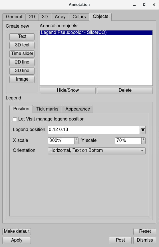
- Click Objects tab where it should have a colorbar object (Legend:Pseudocolor - Slice(CO)).
- Uncheck "Let VisIt manage legend position".
- Change Legend position from (0.05, 0.9) to (0.12 0.13).
- Change X scale from 100% to 300%.
- Change Y scale from 100% to 70%.
- Change Origentation from "Vertical, Text on Right" to "Horizontal, Text on Bottom".
- Click Apply.
- You can also change the number of ticks, tick values, and labels from the "Tick marks" tab.
- Click Appearance tab.
- Uncheck "Draw title" and "Draw min/max" to remove text information.
- Change Font height from "0.015" to "0.04"
- Change Font family from "Arial" to "Times"
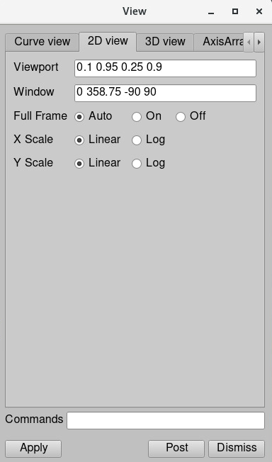
- Let's move the main plot. Open View window by clicking Controls -> View.
- Change Viewport from (0.2 0.95 0.15 0.95) to (0.1, 0.95, 0.25, 0.9).
- Click Apply.
Now the plot will look like this.

Adding coastlines
Downloading shape files
One downside of using VisIt is it doesn't support built-in coastlines. So we have to add coastlines manually. Fortunately, VisIt can easily read shape files (.shp) that used to draw coastlines in various libraries (e.g., basemap, cartopy). You can download shape files from several places publicly available on the web. We list here two popular dataset:
- GSHHS: https://www.ngdc.noaa.gov/mgg/shorelines/gshhs.html
- Natural Earth Data: https://www.naturalearthdata.com/downloads/
A longitude range of the shape files is usually from -180 to 180 degrees. This is good enough for some chemistry models using a longitude range of -180 to 180 degrees (e.g., GEOS-Chem), but CESM/CAM-chem uses a longitude range of 0 to 360 degrees. You can shift the simulated variables around 180 degrees on your own, but we processed the shape file in case you don't want to process the CESM/CAM-chem output. You can download this shape file that has a longitude range of 0 to 360 degrees (use Save link as... option if it opens a new tab with broken letters). This file has been processed from "ne_110m_coastline.shp" file from the Natural Earth Data.
Adding coastlines in the plot
Make sure you have the shape file in your directory. And let's go back to the main window.
- Open -> select "ne_110m_coastline_0_360.shp" -> click OK.
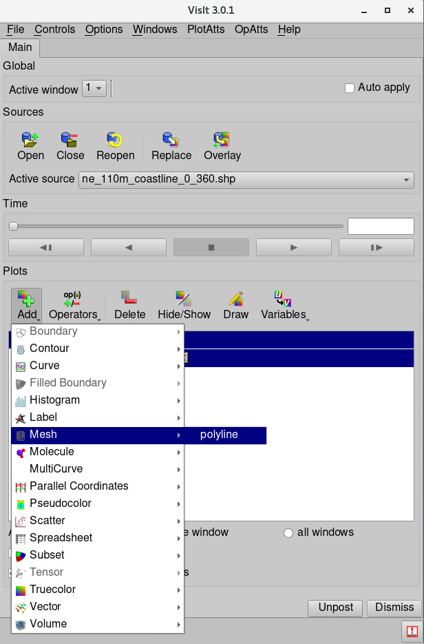
- Now you can find that Active source is changed from "sample.nc" to "ne_110m_coastline_0_360.shp".
- Uncheck "Apply operators to all plot" so that you don't apply "Slice" operator to the coastlines.
- Click on the Add icon -> Mesh -> polyline.
- Then you should have two items in the "Plots" area like below.
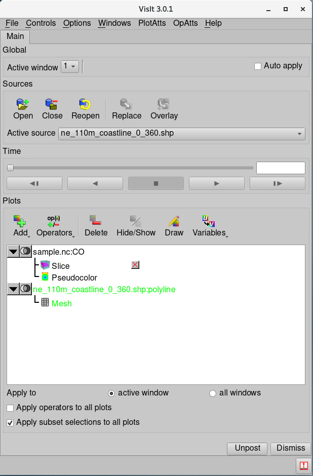
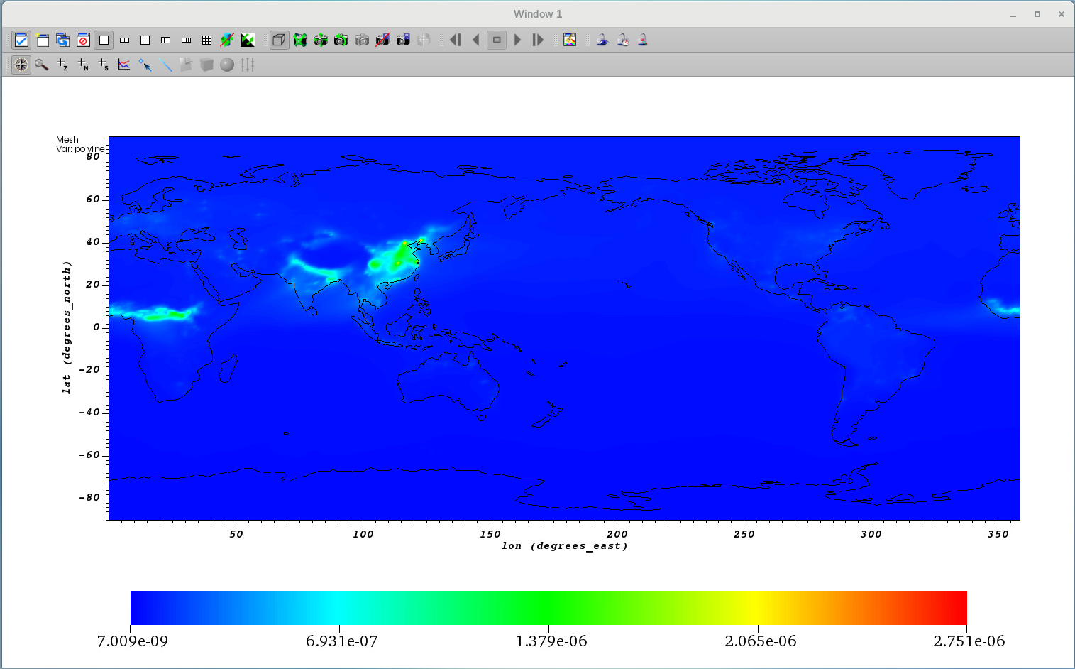
- Click on the Draw button to plot coastlines.
- Now you can see this plot.
- There is a new annotation in the upper left. Let's remove it. Open the Annotation window again.
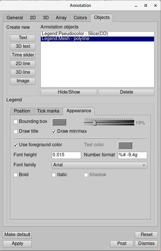
- Select "Legend:Mesh - polyline".
- Click on Appearance tab -> uncheck "Draw title"
- You're all set! Now you have coastlines with CO concentrations!

Using Expressions to create new variables for visualizations
You can create new variables that can be used in visualizations via Expression window. Let's try a simple example here. For various usage and functions see this VisIt manual for Expressions. In this example, we are going to multiply 1e9 to make CO concentrations from mol/mol to ppbv.
- Open Expressions window: Click Controls -> Expressions.
- Click on the New button.
- Change Name from "unnamed1" to "CO_ppbv".
- Add "CO * 1e9" in the Standard editor.
- Click Apply.
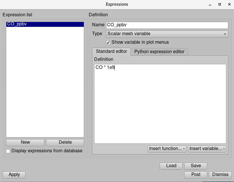
Now you have a new variable named "CO_ppbv". Let's plot a new variable instead of an original one.
- Go back to the main window
- Change Active source from "ne_110m_coastline_0_360.shp" to "sample.nc".
- Select "sample.nc:CO", and then click on the Variables button.
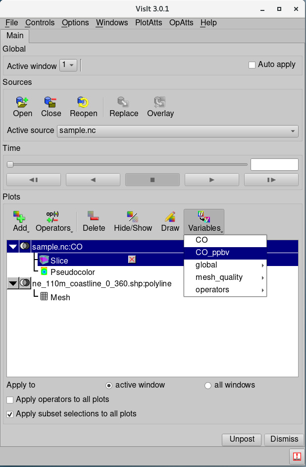
- Click "CO_ppbv" variable, then the plot will be immediately updated (see the tick values in the colorbar).

Finishing touch
Changing longitude and latitude fonts, adding grid lines
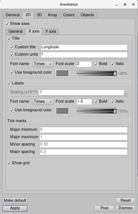
- Open Annotation window again (Controls -> Annotation).
- Click the 2D tab and then go to the X axis.
- Click Custom title and units, and put "Longitude" and "º".
- Under the Title section, change Font name from Courier to Times, and set Font scale to 2.
- Under the Labels section, change Font name from Courier to Times, and set Font scale to 1.5.
- Check Show grid.
- Click Apply.
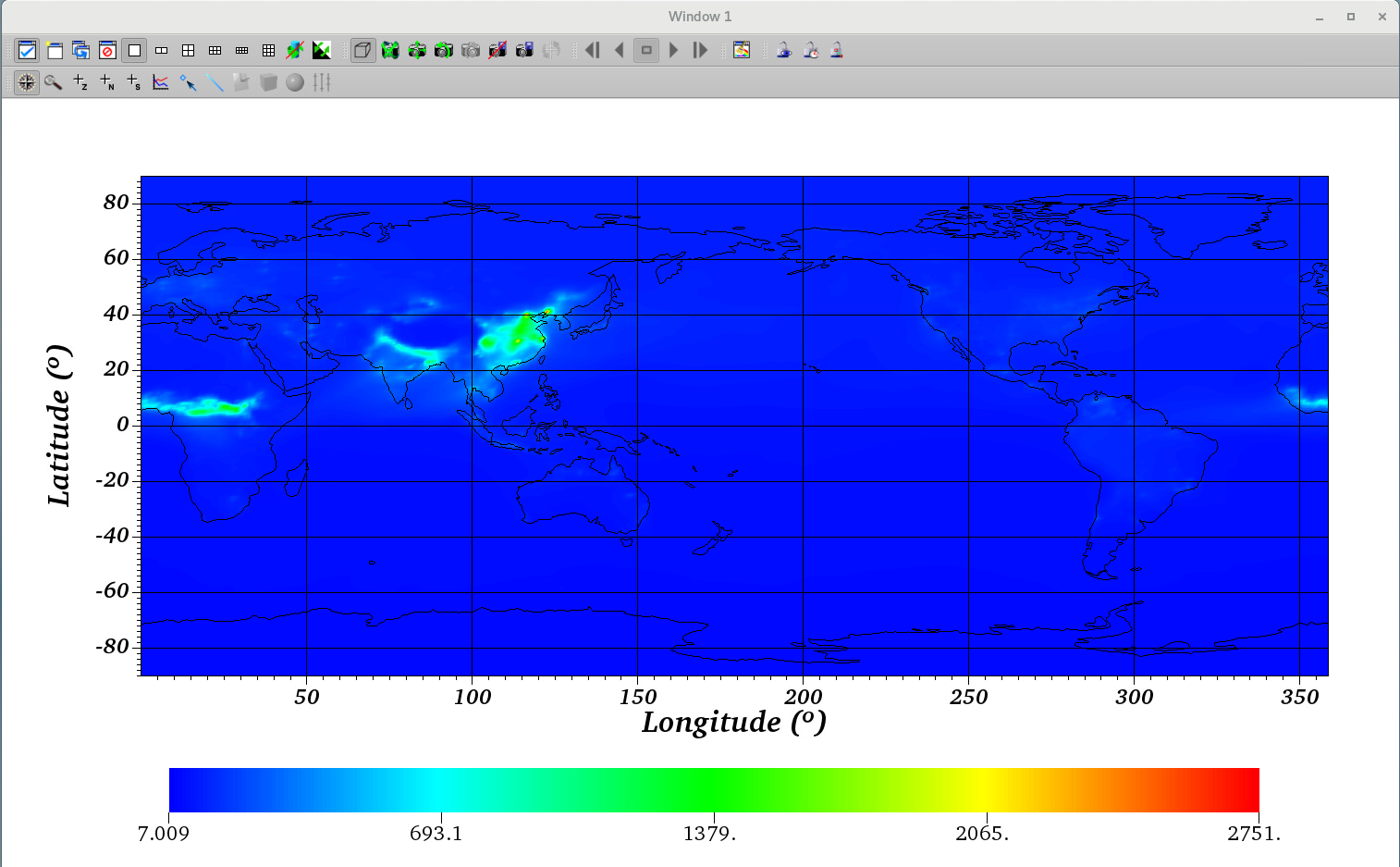
- Do the same process above for Y axis, but with a custom title of Latitude.
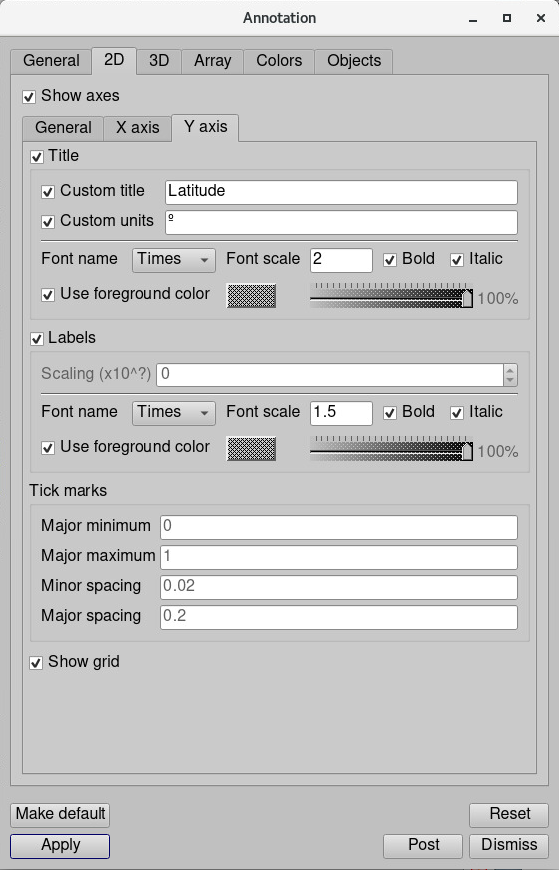
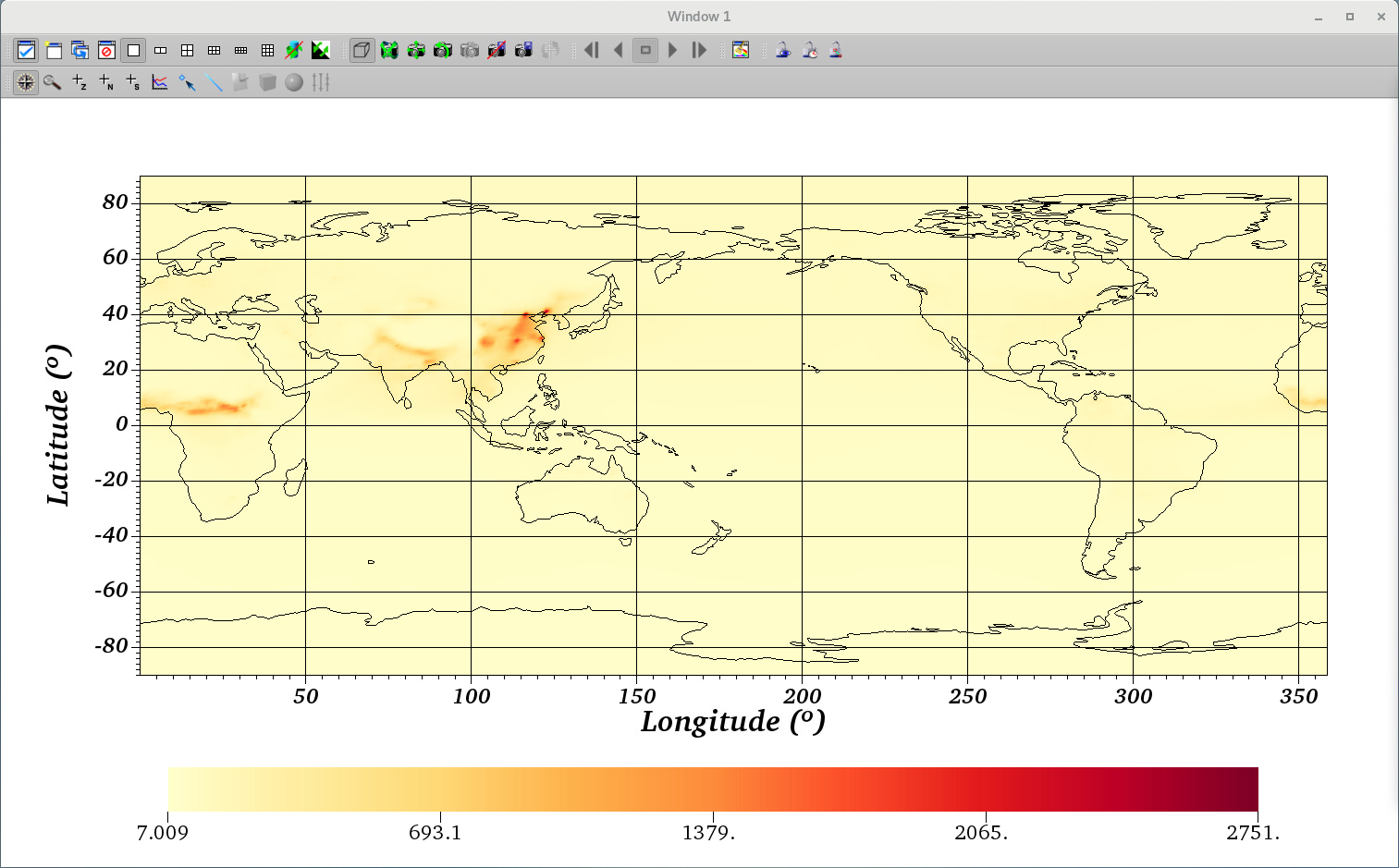
You will get the plot like this.
Changing a color table
Changing color tables or creating a new color table (either discrete or continuous) is very straightforward in VisIt. Let's change the color table in this example.
- Click Controls -> Color table to open "Color tables" window.
- Click on the hot button. It will open the available color tables you have. Click anyone you want but we will use "YlOrRd" in this example.
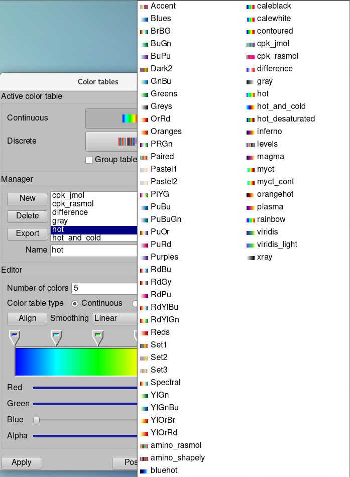
- Click Apply.
- The colors in the plot will be immediately changed. You can also make a new color table easily by clicking on the New button under the Manager section.
Changing a color scale from linear to log
- Click PlotAtts -> Pseudocolor to open the "Pseudocolor plot attributes" window.
- Click the Log ratio button.
- If you want, check the Minimum and Maximum under the Limits section, and provide the min/max values you want for your plot.
- Click Apply
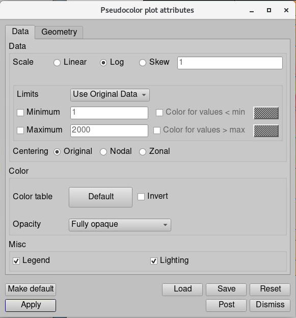
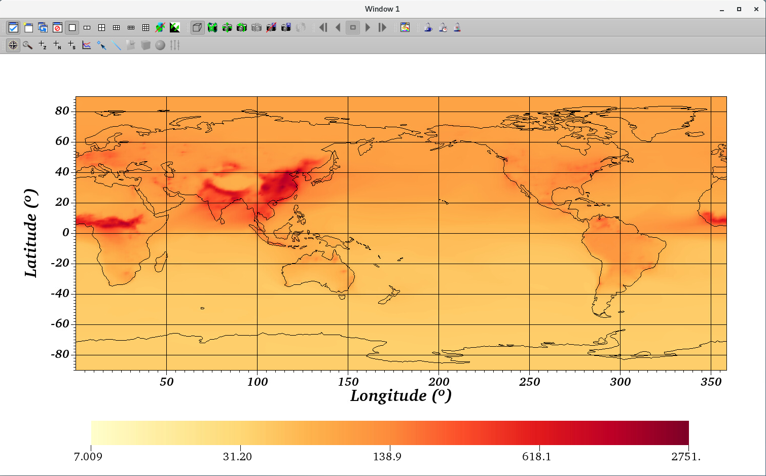
You will get a plot like below.
Adding a title
- Open Annotation window again (Controls -> Annotation).
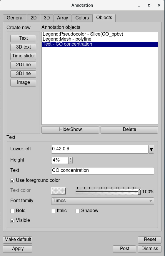
- Go to the Objects tab.
- Click on the Text button on the left under Create new section.
- A small window will pop up with a name. This name is used for the command line interface. Click OK.
- You will get the third annotation objects - "Text - 2D text annotation", and you can also find "2D text annotation" in the middle of the plot.
- Change the "Lower Left" values from (0.5 0.5) to (0.42 0.9).
- Change the "Height" from 3% to 4%.
- Change the "Text" from "2D text annotation" to "CO concentration".
- Change the "Font family" from "Arial" to "Times".
- Click Apply.
- Note that you can also add a unit with the same process above.
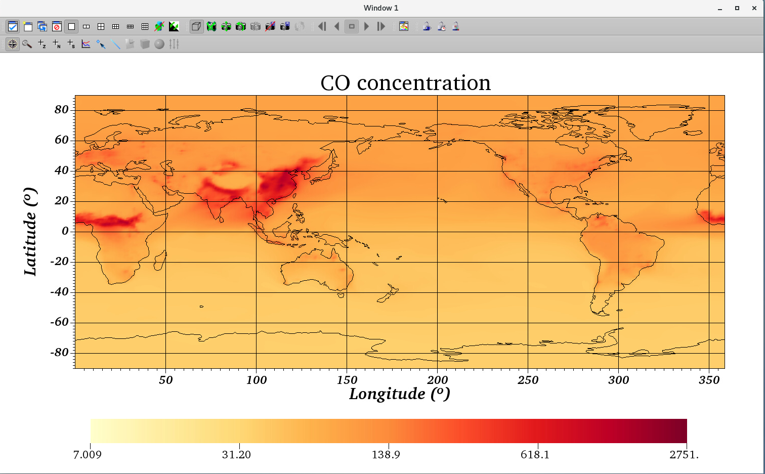
This is the final plot in this example.
Navigating the plot - Moving and Zooming in/out
Navigating the plot is interactive and intuitive. You can use your mouse to navigate the plot. See the video for example below. Note that Longitude and Latitude values are changed accordingly as you navigate the plot.
Getting information from the plot
Getting a value (and coordinates) underneath the mouse cursor
VisIt provides a way to interactively pick values from the visualized data using the visualization window's Zone Pick and Node Pick modes. When a visualization window is in one of those pick modes, each mouse click in the visualization window causes VisIt to find the location and values of selected variables at the pick point. When VisIt is in Zone pick mode, it finds the variable values for the zones that you click on. When VisIt is in node pick mode, similar information is returned but instead of returning information about the zone that you clicked on, VisIt returns information about the node closest to the point that you clicked. Let's get a taste of it below. For more details, see this official VisIt manual page.
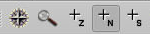
- Click the +N icon. It is located in the upper left corner of your plot window.
- Click any point on your map to get longitude, latitude, and CO concentrations.
- Below is the demonstration that shows how to pick points.
Getting one dimensional curve from point A to point B
You can use a lineout mode, which is essentially a slice of a two-dimensional dataset that produces a one dimensional curve in another window. When a visualization window is in lineout mode, pressing the left mouse button in the window creates the first endpoint of a line that will be used to create a curve. As you move the mouse around, the line to be created is drawn to indicate where the lineout will be applied. When you release the mouse button, VisIt adds a lineout to the window and a curve plot is created in another window. See the demonstration below.
Saving and restoring
Saving session files
Once you have set up your plots, you can select "Save session" or "Save session as" option in the Main Window’s File menu to open up a Save session dialog. Once the Save session dialog is opened, select the location and filename that you want to use to store the session file. Once you select the location and filename to use when saving the session file, VisIt writes an XML description of the complete state of all visualization windows, plots, and GUI windows into the session file so the next time you come into VisIt, you can completely restore your VisIt session.
Restoring session
After restoring a session file, VisIt will look exactly like it did when the session file was saved. To restore a session file, click the Restore session option from the Main Window’s File menu to open an Open session file dialog. Choose a session file to open using the Open file dialog. Once a file is chosen, VisIt restores the session using the selected session file.
Saving the plot (visualization window)
VisIt allows you to save the contents of any open visualization window to a variety of file formats. You can save visualizations as images so they can be imported into presentations. Alternatively, you can save the geometry of the plots in the visualization window so it can be imported into other computer modeling and visualization programs.
VisIt currently supports the image files formats: BMP, JPEG, PNG, PPM, Raster Postscript, RGB, and TIFF.
VisIt currently supports the geometry file formats: Curve, Alias WaveFront Obj, PLY, POV, STL, ULTRA, and VTK.
Click the Save window option from the Main Window's File menu. Note that you can set save options before saving, including filename, file type, aspect ratio, pixel data, etc.
Scripting - if you prefer command line interface to graphical user interface
Modelers usually use the command line interface (e.g., IDL, NCL, python, Matlab, etc.) rather than the graphical user interface. VisIt also supports the command line interface through the Python scripting language. You can see more in-depth tutorial and usage of functions from the official VisIt python interface manual. However, you may need significant time to get the exact function/code you want to have, because VisIt is designed for general scientific applications in addition to atmospheric sciences. There are ways to get the corresponding code from your GUI actions.
WriteScript function
WriteScript function will create a python script that describes all of your current plots. This function is meant to be able to write out the current state of VisIt to a Python script that can be used later to reproduce a visualization. So, after you completed your plot, you don't have to redo all the GUI actions for the same plot with different variables!
- Click Controls -> Command to open Commands window
Put these lines in the Commands.
f = open("script.py", "wt") WriteScript(f) f.close()- Click on the Execute button.
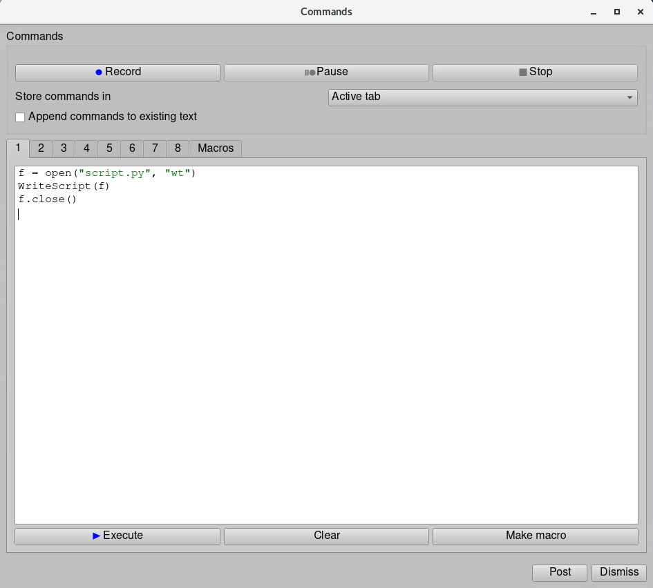
- You will be able to find script.py file created in your directory. You may want to edit the resulting script file since it may be verbose, depending on how many plots you have or the complexity of the data file. But at least, you will be able to find the commands needed to be provided for your plot with some comments in the file.
Recording GUI actions to python scripts
VisIt's Commands window provides a mechanism to translate GUI actions into their equivalent Python commands.
- Open the Commands window again by selecting Controls → Command.
- Click the Record button.
- Perform GUI actions - in this example, let's change minimum and maximum of the plot data to 1 and 2000 (hint: you can change these values in "Pseudocolor plot attributes" window.
- Return to the Commands window, and click the Stop button.
The equivalent Python script will be placed in the tab in the Commands window. The results will look like this.
Reconding GUI actions to Python scriptsPseudocolorAtts = PseudocolorAttributes() PseudocolorAtts.scaling = PseudocolorAtts.Log # Linear, Log, Skew PseudocolorAtts.skewFactor = 1 PseudocolorAtts.limitsMode = PseudocolorAtts.OriginalData # OriginalData, CurrentPlot PseudocolorAtts.minFlag = 1 PseudocolorAtts.min = 1 PseudocolorAtts.useBelowMinColor = 0 PseudocolorAtts.belowMinColor = (0, 0, 0, 255) PseudocolorAtts.maxFlag = 1 PseudocolorAtts.max = 2000 PseudocolorAtts.useAboveMaxColor = 0 PseudocolorAtts.aboveMaxColor = (0, 0, 0, 255) PseudocolorAtts.centering = PseudocolorAtts.Natural # Natural, Nodal, Zonal PseudocolorAtts.colorTableName = "Default" PseudocolorAtts.invertColorTable = 0 PseudocolorAtts.opacityType = PseudocolorAtts.FullyOpaque # ColorTable, FullyOpaque, Constant, Ramp, VariableRange PseudocolorAtts.opacityVariable = "" PseudocolorAtts.opacity = 1 PseudocolorAtts.opacityVarMin = 0 PseudocolorAtts.opacityVarMax = 1 PseudocolorAtts.opacityVarMinFlag = 0 PseudocolorAtts.opacityVarMaxFlag = 0 PseudocolorAtts.pointSize = 0.05 PseudocolorAtts.pointType = PseudocolorAtts.Point # Box, Axis, Icosahedron, Octahedron, Tetrahedron, SphereGeometry, Point, Sphere PseudocolorAtts.pointSizeVarEnabled = 0 PseudocolorAtts.pointSizeVar = "default" PseudocolorAtts.pointSizePixels = 2 PseudocolorAtts.lineType = PseudocolorAtts.Line # Line, Tube, Ribbon PseudocolorAtts.lineWidth = 0 PseudocolorAtts.tubeResolution = 10 PseudocolorAtts.tubeRadiusSizeType = PseudocolorAtts.FractionOfBBox # Absolute, FractionOfBBox PseudocolorAtts.tubeRadiusAbsolute = 0.125 PseudocolorAtts.tubeRadiusBBox = 0.005 PseudocolorAtts.tubeRadiusVarEnabled = 0 PseudocolorAtts.tubeRadiusVar = "" PseudocolorAtts.tubeRadiusVarRatio = 10 PseudocolorAtts.tailStyle = PseudocolorAtts.None # None, Spheres, Cones PseudocolorAtts.headStyle = PseudocolorAtts.None # None, Spheres, Cones PseudocolorAtts.endPointRadiusSizeType = PseudocolorAtts.FractionOfBBox # Absolute, FractionOfBBox PseudocolorAtts.endPointRadiusAbsolute = 0.125 PseudocolorAtts.endPointRadiusBBox = 0.05 PseudocolorAtts.endPointResolution = 10 PseudocolorAtts.endPointRatio = 5 PseudocolorAtts.endPointRadiusVarEnabled = 0 PseudocolorAtts.endPointRadiusVar = "" PseudocolorAtts.endPointRadiusVarRatio = 10 PseudocolorAtts.renderSurfaces = 1 PseudocolorAtts.renderWireframe = 0 PseudocolorAtts.renderPoints = 0 PseudocolorAtts.smoothingLevel = 0 PseudocolorAtts.legendFlag = 1 PseudocolorAtts.lightingFlag = 1 PseudocolorAtts.wireframeColor = (0, 0, 0, 0) PseudocolorAtts.pointColor = (0, 0, 0, 0) SetPlotOptions(PseudocolorAtts)
- Note that the scripts can be very verbose and contain some unnecessary commands, which can be edited out.
Drawing a map on an unstructured grid - MUSICA output
Installing the VisIt plugin to view unstructured grid
The CESM/CAM-chem with regional refinement (aka MUSICA-V0) will save results on an unstructured grid mesh. If you read a NetCDF file output without the plugin installed in this chapter, you will see the 2D plot with "lev" vs "ncol" on the Y and X-axis, which you will not want to draw. We have to let VisIt know latitude and longitude values for each "ncol" element, please follow the installation instructions below.
(1) Copy the spectral element reader plugin
(1-1) If you have access to Cheyenne or Casper, copy this directory:
/glade/scratch/patc/MUSICA_DEMO_NOV20/Demo_Files/VisIt_plugin/MyPlugins/NETCDF_For3.1.3
If the files don't exist due to the Cheyenne scratch purge policy or for some reason, here is an alternative path: /glade/work/cdswk/Visualization/NETCDF_For3.1.3
(1-2) If you don't have access to Cheyenne or Casper, files are also available from Github:
(2) Run the following to build and install:
(2-1) on Mac
Run the following to build and install:
- VisIt plugin install on Mac
mymac% ~/Desktop/VisIt.app/Contents/Resources/bin/xml2cmake NETCDF.xml
mymac% cmake . # [NOTE THE DOT, IT IS IMPORTANT]
mymac% make
When this is done, the plugin has been installed into your local directory. ~/.visit/:
- Check whether the plugin is correctly installed
mymac% ls ~/.visit/3.1.3/darwin-x86_64/plugins/databases/lib*
/Users/YOU/.visit/3.1.3/darwin-x86_64/plugins/databases/libENETCDFDatabase_par.dylib
/Users/YOU/.visit/3.1.3/darwin-x86_64/plugins/databases/libENETCDFDatabase_ser.dylib
/Users/YOU/.visit/3.1.3/darwin-x86_64/plugins/databases/libINETCDFDatabase.dylib
/Users/YOU/.visit/3.1.3/darwin-x86_64/plugins/databases/libMNETCDFDatabase.dylib
(2-2) on Casper
Basically, you have to follow the same steps as above, but you may encounter the error due to a library compatibility issue. So, first check the libraries when VisIt was installed on Casper. As of 15-Jan-2021, these are what you can find:
- VisIt module check on Casper
Capser$ module load visit
Capser$ module help visit

---------------------------- Module Specific Help for "visit/3.0.1" ----------------------------
VisIt is an Open Source, interactive, scalable, visualization, animation
and analysis tool.

Advanced visualization applications such as VisIt should be launched in
a TurboVNC session on the DAV machines.

Software website - https://wci.llnl.gov/simulation/computer-codes/visit/

Built on Wed Aug 28 14:55:55 MDT 2019
Modules used:
   ncarenv/1.2
   gnu/7.3.0
   openmpi/3.1.3
As of 15-Jan-2021, these are default modules on Casper:
- Default modules on Capser as of 15-Jan-2021
Capser$ module list

Currently Loaded Modules:
  1) ncarenv/1.3    3) ncarcompilers/0.5.0   5) netcdf/4.7.4
  2) intel/19.0.5   4) openmpi/4.0.5         6) visit/3.0.1
Let's change the loaded module versions to make them the same (or at least there are not many differences in versions, as close as possible) as the modules when the VisIt was installed on Casper.
- Default module change on Casper
Casper$ module load ncarenv/1.2  # ncarenv/1.3 -> ncarenv/1.2

The following have been reloaded with a version change:
  1) ncarenv/1.3 => ncarenv/1.2


Casper$ module load gnu/7.3.0   # intel/19.0.5 -> gnu/7.3.0

Lmod is automatically replacing "intel/19.0.5" with "gnu/7.3.0".


Inactive Modules:
  1) ncarcompilers/0.5     2) netcdf/4.7.4     3) openmpi/4.0.5


Casper$ module load openmpi/3.1.4   # openmpi/4.0.5 -> openmpi/3.1.4, openmpi/3.1.3 in not available as of 15-Jan-2021

Activating Modules:
  1) openmpi/3.1.4


Casper$ module list

Currently Loaded Modules:
  1) visit/3.0.1   2) ncarenv/1.2   3) gnu/7.3.0   4) openmpi/3.1.4

Inactive Modules:
  1) ncarcompilers/0.5   2) netcdf/4.7.4
Now you have the correct library that will not make an error while installing the plugin. Do the same process in (2-1), like below.
- VisIt plugin install on Casper
Casper$ cd {your NETCDF plugin directory}
Casper$ rm -f CMakeCache.txt # in case you have the permission error
Casper$ rm -f CMakeLists.txt # in case you have the permission error
Casper$ xml2cmake NETCDF.xml
Casper$ cmake . # [NOTE THE DOT, IT IS IMPORTANT]
Casper$ make
Let's check whether the plugin is correctly installed. You have to have these four files in your .visit directory like below.
- Check whether the plugin is correctly installed
Casper$ cd /glade/u/home/{Your Casper ID}/.visit/3.0.1/linux-x86_64/plugins/databases
Casper$ ls
libENETCDFDatabase_par.so  libINETCDFDatabase.so  libENETCDFDatabase_ser.so  libMNETCDFDatabase.so
Note that versions in the above example can be changed in the future as CISL continuously updates libraries and modules.
Putting the connectivity data needed for displaying unstructured grid model output
The connectivity data needed for displaying model output is not included in CESM history filles, so it must be supplied separately. The needed information is embedded into the LATLON grid files that should be already created by Gen_ControlVolumes.exe program, so all that needs to be done is to add a renamed copy of this file into your ~/.visit directory:
mymac/casper$ cp $(MUSICA_REPO)/grids/{YOUR_GRID_name}_LATLON.nc ~/.visit/ SEMapping_nnnnnnnn.nc
Here is an example:
casper$ pwd
/glade/u/home/cdswk/.visit


casper$ ncdump -h /glade/work/cdswk/VRM_Files/ne0np4.KORUS03.ne30x16/grids/KORUS03.ne30x16_np4_LATLON.nc
netcdf KORUS03.ne30x16_np4_LATLON {
dimensions:
	ncol = 97418 ; ## <===== THIS NUMBER SHOULD BE USED FOR YOUR SEMapping file!! =====
	ncorners = 4 ;
	ncenters = 97416 ;
variables:
	double lat(ncol) ;
		lat:long_name = "column latitude" ;
		lat:units = "degrees_north" ;
	double lon(ncol) ;
		lon:long_name = "column longitude" ;
		lon:units = "degrees_east" ;
	double area(ncol) ;
		area:long_name = "area weights" ;
		area:units = "radians^2" ;
	int element_corners(ncorners, ncenters) ;

// global attributes:
		:Grid = "Variable Resolution: KORUS03.ne30x16_EXODUS.nc" ;
		:Created\ by = "Gen_ControlVolumes.exe" ;
}


casper$ cp /glade/work/cdswk/VRM_Files/ne0np4.KORUS03.ne30x16/grids/KORUS03.ne30x16_np4_LATLON.nc ./SEMapping_00097418.nc
Where the 8 digit index for the SEMapping file is the value of ncol for the grid. The reader will does not currently have a prompt for the user to specify this file. It just constructs a file name based on the grids size and looks here for it. It is cumbersome, but it works for now, as long as you don't have 2 grids with the same ncol value!
The LATLON file for the CONUS grid released in CESM2.2 is: /glade/p/acom/MUSICA/grids/ne0CONUSne30x8/ne0CONUS_ne30x8_np4_LATLON.nc (linked to SEMapping_00174098.nc).
There is an effort to make CESM files self-describing as of 15-Jan-2021. When/if the revision is done, then this version of the plugin will likely become obsolete and need to be updated.