According to the Licor 7500 manual, there is a 0.186 second sampling lag in the 7500. This can be increased with an output delay parameter, so that it can be synchronized with the sampling of a sonic. I've verified that the output delays on our 7500's are set to 0. Since the CSAT3 and Licor operate asynchronously, there is no advantage in further adjustment of the Licor delay to be a multiple of the CSAT3 sample period.
We have not been incorporating a 7500 lag in our data processing. We do correct for the 2 sample delay of the CSAT3 sonics. Subtracting 0.186 seconds from the 7500 samples does increase the correlation and fluxes between w and h2o and co2.
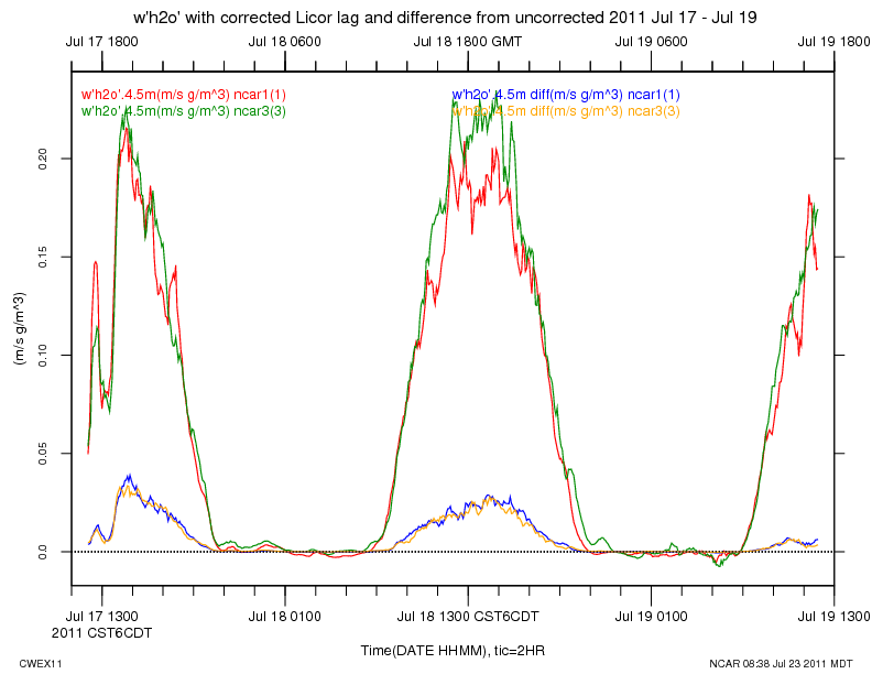
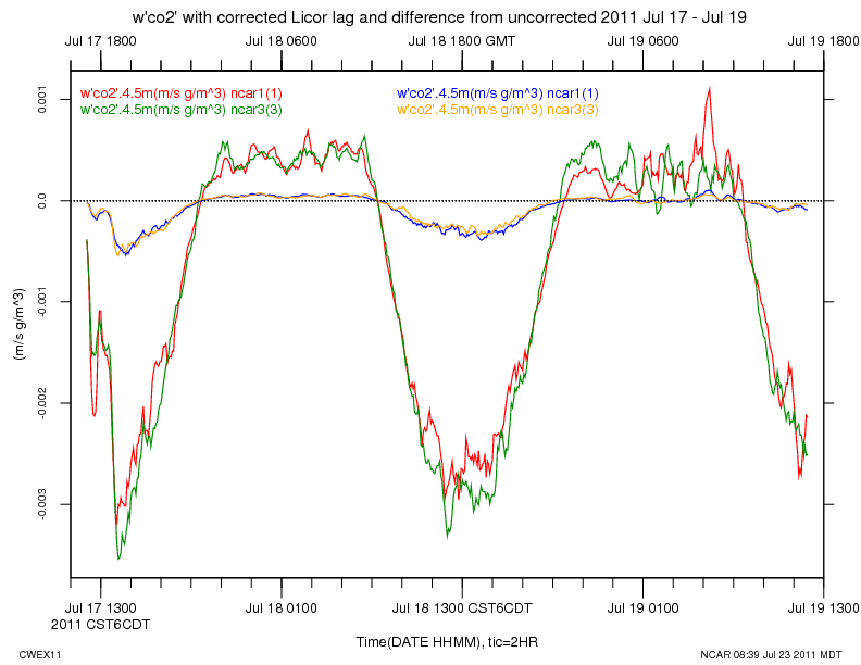
The w'h2o' and w'co2' fluxes increase by about 15% when a lag of 0.186 is applied to the Licor data. These plots are of the corrected flux and the difference between the corrected and uncorrected fluxes, for 2 days, centered on Jul 18:
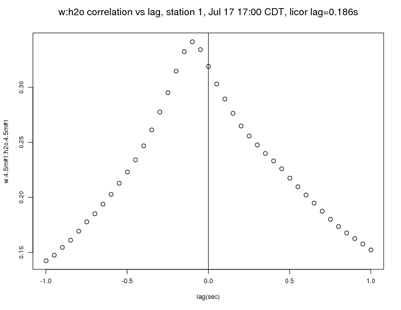
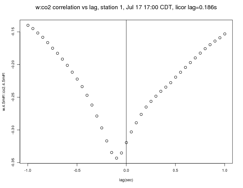
Here are the correlation vs lag plots between w and h2o and co2 from station 1 for Jul 17, 17:00 - 17:30 CDT. The wind was out of the south at this time:
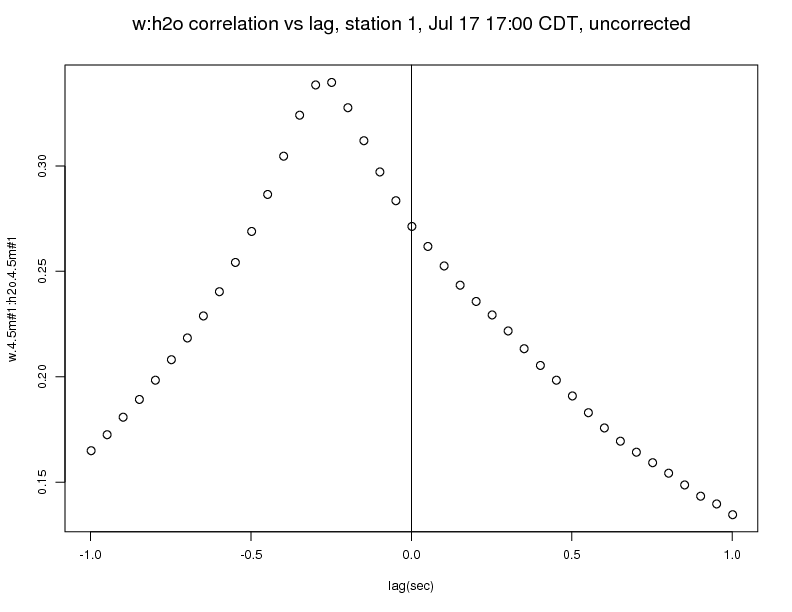
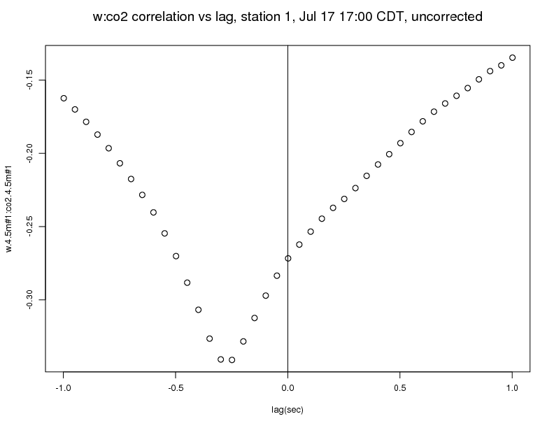
After applying a 0.186 second lag to the Licor data, you can see that the correction is in the right direction, but there is still a lag of about 2 samples, 0.1 seconds:
(It pays to read the manual!)
For future reference, here is the splus code to plot the correlations:
dpar(start="2011 jul 17 17:00",lenmin=30,stns=1)
iod = prep(c("w.4.5m#1","h2o.4.5m#1","co2.4.5m#1"),rate=20)
x = readts(iod)
close(iod)
cwh = crosscorr(x[,1:2],lags=c(-1,1))
plot(as.numeric(utime(positions(cwh))),cwh,xlab="lag(sec)",ylab="w.4.5m#1:co2.4.5m#1")