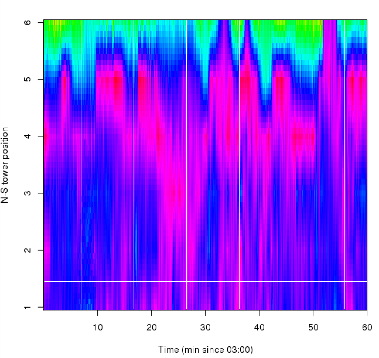
For my own records, 4 hours of data have been analyzed so far from Christoph's system: 11/20-21: 0300-0700Z. This shows a cold air microfront of several degrees with an axis most of the way up the north slope of the gully, in conditions with Northwest winds. Occasionally, the front makes it to the top of the North slope. Attached is a simulation for the first hour of what the fiber sees (albeit with much higher spatial resolution) using sonic tc data.
Screen Shot 2015-05-21 at 5.29.53 PM.png
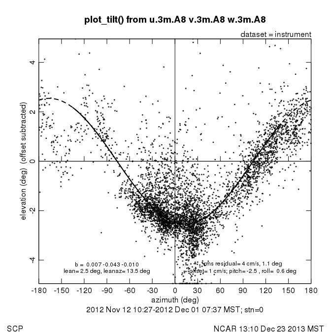
dpar(start="2012 Nov 12 00:00",lenday=20,stns=0,hts=3,sfxs="A8")
dataset("instrument")
plot_tilt()
Added these values to geo_tilt_cor/irgason_a8.dat: woff=-0.01, lean=2.5, leanaz=13.5
Prior to deployment of the Handar sonics in the SCP field program, we tested the Handar 2D sonics in the EOL wind tunnel, which has a test section with a circular cross-section 1m in diameter. Wind speed and direction measured by the sonic were compared to tunnel speed measured by a pitot-static tube and wind direction measured by the orientation of the sonic in the wind tunnel. Each sonic was rotated through 360 degrees in 15 degree increments for tunnel speeds of 2, 5, 10, 15, 20, and 25 m/s. A subset of three sonics was also rotated in 3 degree increments.
The following table lists the gain, offset, and rms residuals (as a per cent of the pitot speed) from a least-squares fit of the sonic speed as a function of the tunnel (pitot) speed,
sonic speed = gain x pitot speed + offset.
The last column lists the rms residuals of a linear fit of sonic direction as a function of sonic orientation in the wind tunnel.
| SN | Date | spd gain | spd offset | spd rms | dir rms |
|---|---|---|---|---|---|
| 00194 | 8/20/12 | 1.04 | -5 cm/s | 3% | 0.5 deg |
| 00678 | 8/15/12 | 1.03 | -4 cm/s | 3% | 0.8 deg |
| 00719 | 8/13/12 | 1.04 | -6 cm/s | 3% | 0.9 deg |
| 01528 | 8/14/12 | 1.03 | -4 cm/s | 3% | 0.8 deg |
| 01627 | 8/16/12 | 1.03 | +4 cm/s | 3% | 0.9 deg |
| 01627 | 8/21/12 | 1.03 | -3 cm/s | 3% | 1.1 deg |
| 01631 | 8/14/12 | 1.03 | -4 cm/s | 2% | 0.8 deg |
| 01660 | 8/13/12 | 1.03 | -4 cm/s | 3% | 0.8 deg |
| a0730003 | 8/15/12 | 1.03 | -4 cm/s | 3% | 1.9 deg |
| y384003 | 8/14/12 | 1.03 | 0 cm/s | 2% | 2.8 deg |
The TRH sensors were run through the calibration lab after SCP. Temperatures were checked over the range of -20C to 30C. RH was checked over the range of 10% to 90% at a temperature of 7C. The table below presents the mean error, Sensor - Ref, and the minimum and maximum error.
For humidity, in the cases where the range of the error is large, the errors typically increase systematically from the smallest errors around 10% RH to the largest errors around 90% RH.
Loading
I added new "slope" coefficients to the Rpile_in.dat and Rpile_out.dat cal files to change their calibration coefficients from those measured in March 2011 in the NOAA blackbody to those determined by comparison (March 1-April 1, 2013) to two EOL CG4s calibrated at NREL in August 2012 and traceable to the World Infrared Standards Group (WISG) at the World Radiation Center in Davos, Switzerland.
Rpile_in (SN 100225) changed from 11.28 uV per W/m^2 to 11.12 uV per W/m^2; cal file slope = 1.014
Rpile_out (SN 100226) changed from 11.81 uV per W/m^2 to 10.76 uV per W/m^2; cal file slope = 1.005
I just ran the 3 ECHO probes used during SCP through a beaker of sand with various amounts of moisture (manually mixed in). The results are:
Variable |
Qsoil.g |
Qsoil.c |
Qsoil.c2 |
|---|---|---|---|
S/N |
ECHO 001 |
ECHO 002 |
ECHO 012 |
ID |
28 |
29 |
2A |
0ml/2700ml = 0% |
-3.14 |
-2.95 |
-2.33 |
200/2800 = 7.1% |
3.71 |
3.91 |
4.17 |
400/2900 = 13.8% |
15.87 |
16.00 |
16.30 |
600/2900 = 20.7% |
21.05 |
22.21 |
24.02 |
800/2800 = 28.6% |
25.33 |
25.78 |
29.12 |
This suggests that there are small gain/bias errors that have probe 001 read lower that probe 002 which is lower than 012 -- in other words, an order of 001/002/012
However, the one set of gravimetric samples showed that probe 001 was within 1% of its gravimetric sample, whereas probe 002 was 2% high and probe 012 was 3% low. This would imply that the order was 012/001/002.
Furthermore, the data consistently show an order 012/002/001, though 001 being larger undoubtedly is real.
I am forced to conclude that 002 reading higher than 012 in the field is not a calibration difference. Thus, this difference must have been due to spatial inhomogeneity in the soil.
For my records, here is code to plot this:
ref = c(0,7.1,13.8,20.7,28.6)
e01 = c(-3.14,3.71,15.87,21.05,25.33)
e02 = c(-2.95,3.91,16.00,22.21,25.78)
e12 = c(-2.33,4.17,16.3,24.02,29.12)
matplot(ref,cbind(e01,e02,e12),xlim=c(-5,30),ylim=c(-5,30))
abline(h=0,v=0)
abline(0,1)
Began January 9, 2013
Following the SCP project, we tested each sonic in a zero-wind enclosure within the EOL temperature chamber, measuring wind component offsets and sonic temperature errors over the nominal range -30 C to 55 C. The procedure is to warm the chamber up to 55 C and then slowly decrease the temperature linearly to -30 C, followed by slowly increasing the temperature back to 55 C. The zero-wind enclosure holds two sonic heads on their sides (with the v-axis vertical) and electronics, one above the other and separated with a horizontal layer of rigid blue foam. On the cool-down cycle, the atmosphere around the top sonic is unstably stratified (cold enclosure lid above warmer air) and that around the bottom sonic is stably stratified (cold enclosure bottom below warmer air). The opposite is true during the warm-up cycle. Both the wind component data and the sonic temperature data have significantly less variance when the air is stably stratified, and thus we use data from the bottom sonic during the cool-down cycle and data from the upper sonic during the warm-up cycle.
The following table shows wind component offsets as okay if the u and v offsets are less than +/- 4 cm/s and the w offsets less than +/- 2 cm/s (between - 20 C and 30 C). If the zero wind offset exceed these thresholds, the table lists the temperature range of the over-limit offset and the largest amplitude of the offset. The plots of offsets versus temperature can then be examined to determine the exact nature of the offset.
The sonic temperature corrections are listed as the slope and offset of a linear fit (between -20 C and 30 C), Tc = offset + slope*tc.sonic, where Tc is calculated from temperature, relative humidity, and pressure measured in the zero-wind enclosure. Rudy also calculated the sonic temperature correction (again from -20 to 30 C) by interpolating the speed-of-sound temperatures of the hygrothermometers to the height of the sonic.
Note that we have repeated the laboratory tests on SN0923 and SN0833 to determine the reproducibility of the results. The velocity component offsets agree within less than 2 cm/s and the temperature offsets agree within 0.06-0.10 C and the slopes agree within 0.2-0.3%, for an overall agreement of no worse than 0.1 C.
SCP Site |
EOL cal |
Sonic |
Owner |
Cal date |
u |
v |
w |
tc offset |
tc slope |
rms dev |
|---|---|---|---|---|---|---|---|---|---|---|
Ah1 |
1/09/13 |
0923 |
UC Davis (KT) |
15aug12 |
ok |
7 - 23 C; |
ok |
0.10 |
1.0223 |
0.07 |
repeat calibration |
1/10/13 |
0923 |
" |
" |
ok |
7 - 23 C; |
ok |
0.04 |
1.0204 |
0.06 |
Ah2 ("glitching in high winds") |
1/09/13 |
0833 |
UC Davis (KT) |
29aug12 |
ok |
ok |
ok |
0.69 |
0.9971 |
0.08 |
repeat calibration |
1/10/13 |
0833 |
" |
" |
ok |
ok |
ok |
0.79 |
0.9938 |
0.08 |
Ah2 (after 10/19/12@10:15) |
2/04b/13 |
0671 |
ISFS |
28jun12 |
ok |
ok |
ok |
-0.13 |
1.0172 |
0.10 |
Aph3 |
1/14/13 |
0743 |
RAL (Gochis) |
05jul12 |
ok |
ok |
ok |
0.15 |
1.0206 |
0.11 |
A4 |
2/06b/13 |
1120 |
ISFS |
19jul12 |
ok |
23 - 30 C; |
ok |
-0.19 |
1.0193 |
0.06 |
Ah5 |
1/14/13 |
0732 |
RAL (Gochis) |
09jul12 |
ok |
ok |
ok |
0.86 |
1.0004 |
0.11 |
Ah6 |
2/07/13 |
0800 |
ISFS |
19jun12 |
ok |
ok |
ok |
0.08 |
1.0156 |
0.08 |
A7 |
2/04/13 |
0673 |
ISFS |
18jul12 |
ok |
ok |
ok |
1.10 |
0.9979 |
0.09 |
Ap8 |
1/11/13 |
0176 |
UC Davis (KT) |
22aug12 |
ok |
ok |
ok |
0.50 |
1.0272 |
0.05 |
Ap9 |
2/05/13 |
1121 |
ISFS |
08dec11 |
ok |
ok |
ok |
-0.63 |
1.0137 |
0.10 |
Ap10 |
2/05/13 |
0677 |
ISFS |
17jul12 |
ok |
ok |
ok |
1.16 |
0.9995 |
0.10 |
Ars11 |
2/07b/12 |
0674 |
ISFS |
13aug12 |
ok |
ok |
ok |
0.96 |
0.9977 |
0.08 |
Ap12 |
2/01/13 |
0855 |
ISFS |
12sep12 |
ok |
ok |
ok |
0.95 |
0.9975 |
0.11 |
A13 |
1/31b/13 |
0745 |
RAL (Gochis) |
09jul12 |
ok |
ok |
ok |
1.21 |
0.9978 |
0.11 |
Ap14 |
2/06b/13 |
1124 |
ISFS |
19jul12 |
ok |
ok |
ok |
0.89 |
1.0048 |
0.08 |
A15 |
2/05b/13 |
1122 |
ISFS |
08dec11 |
ok |
ok |
ok |
-0.44 |
1.0161 |
0.07 |
A16 |
1/30/13 |
0740 |
RAL (Gochis) |
28aug12 |
ok |
ok |
ok |
-1.88 |
0.9979 |
0.06 |
A17 |
2/01/13 |
0856 |
ISFS |
31jan12 |
ok |
19 - 30 C; |
29 - 30 C; |
-0.62 |
1.0145 |
0.10 |
A18 |
1/15/13 |
0744 |
RAL (Gochis) |
05jul12 |
ok |
ok |
ok |
0.41 |
1.0210 |
0.13 |
repeat calibration |
2/07b/13 |
0744 |
" |
" |
ok |
ok |
ok |
0.01 |
1.0227 |
0.06 |
A19 (broken joint; |
|
0672 |
ISFS |
17jul12 |
NA |
NA |
NA |
NA |
NA |
NA |
A19 (installed 9/24/12) |
1/11/13 |
0178 |
UC Davis (KT) |
9sep12 |
ok |
ok |
ok |
0.72 |
1.0001 |
0.10 |
C.1m |
1/07/13 |
0200 |
UC Irvine (JRP) |
27jun12 |
ok |
ok |
ok |
-0.04 |
1.0192 |
0.10 |
C.2m |
1/07/13 |
0197 |
UC Irvine (JRP) |
03jul12 |
ok |
ok |
ok |
0.74 |
0.9900 |
0.07 |
M.05m |
1/15/13 |
1455 |
USFS (WJM) |
29aug12 |
ok |
ok |
ok |
0.66 |
1.0004 |
0.08 |
M.1m |
2/07/13 |
1117 |
ISFS |
08dec11 |
29 - 30 C; |
16 - 27 C; |
ok |
1.06 |
0.9976 |
0.10 |
M.2m (until 9/27/12@15:03?) |
|
0538 |
ISFS |
|
NA |
NA |
NA |
NA |
NA |
NA |
M.2m |
2/04b/13 |
0536 |
ISFS |
27jun12 |
ok |
ok |
ok |
0.80 |
0.9993 |
0.08 |
M.3m |
2/01b/13 |
0540 |
ISFS |
28mar12 |
27 - 30 C; |
ok |
ok |
-0.20 |
0.9930 |
0.15 |
repeat calibration |
2/08/13 |
0540 |
" |
" |
27 - 30 C; |
ok |
ok |
-1.87 |
1.0125 |
0.09 |
M.4m |
1/29/13 |
0738 |
RAL (Gochis) |
29aug12 |
22 - 28 C; |
18 - 25 C; |
ok |
-0.26 |
1.0197 |
0.11 |
M.5m (until 9/27/12@15:03?) |
|
0671 |
ISFS |
|
NA |
NA |
NA |
NA |
NA |
NA |
M.5m |
2/06b/13 |
0537 |
ISFS |
21jun12 |
ok |
ok |
ok |
-0.19 |
1.0134 |
0.09 |
M.10m |
2/01b/13 |
1119 |
ISFS |
09aug12 |
ok |
ok |
ok |
-0.12 |
1.0137 |
0.16 |
repeat calibration |
2/08/13 |
1119 |
" |
" |
ok |
ok |
ok |
1.22 |
0.9969 |
0.09 |
M.20m |
1/31b/13 |
0741 |
RAL (Gochis) |
3jul12 |
ok |
ok |
ok |
-0.09 |
1.0199 |
0.09 |
The 10 Vaisala barometers have been post-cal over the range of 790mb to 850mb in 11 steps.
At each level 30 data points were collected and averaged. The ParoScientific was used as the
reference. The table below shows the results.
Sensor |
mean error (mb) |
stdev (mb) |
||
|---|---|---|---|---|
B1 |
.217 |
0.009643 |
|
|
B2 |
-.022 |
0.022461 |
|
|
B4 |
-.017 |
0.008821 |
|
|
B5 |
-.016 |
0.011472 |
|
|
B6 |
-.053 |
0.008349 |
|
|
B7 |
.005 |
0.005977 |
|
|
B8 |
-.051 |
0.010317 |
|
|
B9 |
-.011 |
0.011812 |
|
|
B10 |
-.001 |
0.009677 |
|
|
4 ParoScientific nano barometers were deployed in SCP. A post-cal was conducted over the range
of 790mb to 840mb in 7 steps. 30 data points were collected at each level.
Sensor |
mean error (mb) |
stdev (mb) |
|---|---|---|
123997 |
0.1563 |
0.161 |
123998 |
0.1930 |
0.184 |
123996 |
0.1974 |
0.184 |
122850 |
0.3316 |
0.184 |
NOTE: 122850 was involved in the lighting strike.

These are the serial numbers of the instruments and their towers during teardown.
Station |
CSAT |
Handar |
Pressure |
OTHER |
|---|---|---|---|---|
Ah1 |
0923 |
000194 |
|
|
Ah2 |
0671 |
01660 |
|
|
Aph3 |
0743 |
y3840003 |
NCAR001 |
|
A4 |
1120 |
|
|
|
Ah5 |
0732 |
123998 |
|
|
Ah6 |
0800 |
00719 |
|
|
A7 |
0673 |
|
|
|
Ap8 |
0176 |
|
B10 |
EC150(1244/1313) |
Ap9 |
1121 |
|
B6 |
|
Ap10 |
0677 |
|
122996 |
|
A11 |
--- |
------- |
------ |
------ |
Ap12 |
0855 |
|
B9 |
|
A13 |
0745 |
|
|
|
Ap14 |
1124 |
|
B5 |
|
A15 |
1122 |
|
|
|
A16 |
0740 |
|
|
|
A17 |
0856 |
|
|
|
A18 |
0744 |
|
|
|
A19 |
--- |
--- |
--- |
--- |
C |
0197,0200 |
|
|
|
|
|
|
|
|
|
|
|
|
|
Main(from bottom): 1455, 1117, 0813(licor), 123997(nano), 0536, 1166(licor), 0540...
Radiation: IN-940185,1002255/ OUT-940187,100226
Grass Soil: ECHO001,H013291,200589,ts001,ts011
Cactus Soil: ECHO002,H992560,200239,ts018,ECHO012
Gordon, Dec 6
Downloaded the remaining archive files from the USB and CF drives.
For stations 1-22 these consisted of the archive files for Dec 1, since the files for Nov 30 and before had been copied to the gully server over the network.
The USB pocketec from gully contained Nov 21 to Dec 1.
The copy_arch_media script also did a fsck on each disk. Some errors were seen and noted below. For the bluetooth Viper systems with CF disks, the number is noted.
stn |
CF |
notes |
|---|---|---|
1 |
20 |
OK |
2 |
26 |
OK |
3 |
|
OK |
4 |
|
OK |
5 |
21 |
OK |
6 |
29 |
OK |
7 |
|
OK |
8 |
24 |
OK |
9 |
22 |
OK |
10 |
27 |
OK |
11 |
|
OK |
12 |
|
OK |
13 |
|
OK |
14 |
28 |
OK |
15 |
|
OK |
16 |
|
fsck errors |
17 |
|
OK |
18 |
|
OK |
19 |
|
many fsck errors |
20 |
|
OK |
21 |
|
24 bad blocks on pocketec |
22 |
|
OK |
Teardown:
Today was very successful. All tower infrastructure is down and all sensors, DSMs removed from the field.
The DSMs and TRHs will be taken back to Boulder Sunday night.
Weather
High cirrus clouds, temp s throughout the night from 0C to 10C. Winds around 3 m/s. History shows winds
pushing 15 m/s during the night.
Status
morning (7:15): Everything looks good tis morning.There were Idiag spikes on about 10 stations last night. I assume due to
high winds. Station 3 shows an RIP in the history.
Starting shutdown @ 7:30am.
Teardown
Stations A1-A7, A15-A19, and C are down. Tomorrow we hope to get the remaining A stations down and the main tower stripped
of sensors and DSM, We will also remove the radiation/soil sensors.
Here are the things that I recall that need to be dealt with:
- Remove radiometer and open-path data (li7500, krypton, ec150) during cleaning events
- Try to recover odd Tsoil.grass data for about a week in early Oct. when scrambled. (Already have code to do this, but might be improved.)
- Remove TRH data when iFan is zero
- Adjust some early TRH data from probes that were swapped based on postcals
- Determine which set of boom angles to use
- Swap Cactus/Grass data from first day
- Determine what to do with Qsoil.c, Qsoil.c2 not matching. Qsoil.c data (when available) are self-consistent from the initial data, even through the lightning. Qsoil.c2 is always lower, but data were reasonable compared to one gravimetric sample. We will measure probe depths to see if this helps explain the differences. (Fix Qsoil probe that dies when cold.)
Weather
Partly cloudy with high cirrus, light winds, <2 m/s. Temperatures a round 0C to 2C.
During the night the winds stayed below 5 m/s.
Status
morning (7:30): All systems running. This is the last day of ops. Teardown will start
tomorrow. I plan to do the final boom angle check today.
afternoon (14:45): Completed shooting angles. Per Steve O. request the boom height of
the EC150 is 2.502m.
Station 17 was showing a few Idiag spikes. I believe this was due to the teardown of Christoph's
equipment.
Cores taken at cactus and then grass at about 1445 today (29 Nov). I brought them back to Boulder and did the first weighing at about 1715, so hopefully they hadn't dried too much. Both samples did not completely fill up the corer (despite being pounded in all the way on the outside). Thus I would estimate that the first core is 0-2.5cm and the second from 2.5-5.5cm.
From the PCAPS entry: The coring tool was set up with two 3cm rings on the top (used) followed by two 1cm rings on the bottom (ignored). Thus, each 3cm sample volume was c(2.5,3)pi(5.31/2)^2=c(55.4,66.4)cm^3.
|
|
Cactus |
Cactus |
Cactus |
Grass |
Grass |
Grass |
|---|---|---|---|---|---|---|---|
Tare |
|
7.945 |
8.000 |
|
8.012 |
7.948 |
|
Wet (including tare) |
|
64.646 |
118.816 |
|
72.906 |
102.492 |
|
Dry (including tare) |
|
61.954 |
110.467 |
|
66.865 |
88.784 |
|
Rho.dry |
dry/vol |
0.98 |
1.54 |
1.28 |
1.06 |
1.22 |
1.15 |
Qsoil (% mass) |
(wet-dry)/wet |
4.75 |
7.53 |
6.59 |
9.31 |
14.50 |
12.39 |
Vol Frac (% vol) |
(wet-dry)*rho.water/vol |
4.86 |
12.57 |
9.06 |
10.91 |
20.63 |
16.21 |
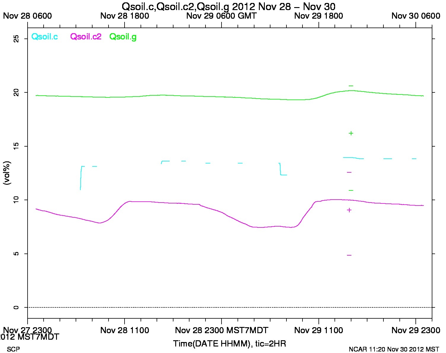
S+ plot:
dpar(start="2012 nov 28 00:00",lenday=2,stns=0)
plot(dat("Qsoil"),ylim=c(0,25))
points(nts(9.06,utime("2012 nov 29 14:45")),col=3,pch="+")
points(nts(c(4.86,12.57),utime(rep("2012 nov 29 14:45",2))),col=3,pch="-")
points(nts(16.21,utime("2012 nov 29 15:00")),col=4,pch="+")
points(nts(c(10.91,20.63),utime(rep("2012 nov 29 15:00",2))),col=4,pch="-")
Resulting plot is below. Both Qsoils are between the values computed for the entire layer (0-5.5cm) and those from the bottom layer (2.5-5.5cm). Note that better agreement might be expected with the bottom layer, since the probe is installed at about 5cm. This is true for Grass, but not quite for Cactus. Also note that the original cactus Qsoil.c probe compares poorer to the gravimetric measurements than the new Qsoil.c2 probe. Overall, these gravimetric data do not suggest that modifying the Qsoil observations is needed.